Using Arbitrary Runge-Kutta Methods (02-runge-kutta)
This example solves the same model problem as the example P03/01-implicit-euler but it shows how arbitrary Runge-Kutta methods can be used for time stepping. Let us begin with a brief introduction to the Runge-Kutta methods and Butcher’s tables before we explain implementation details.
Runge-Kutta methods and Butcher’s tables
Runge-Kutta methods are very nicely described on their Wikipedia page and we recommend the reader to have a brief look there before reading further. In particular, read about the representation of Runge-Kutta methods via Butcher’s tables, and learn how the table looks like if the method is explicit, diagonally-implicit, and fully implicit. You should understand basic properties of Runge-Kutta methods such as that explicit methods always need very small time step or they will blow up, that implicit methods can use much larger time steps, and that among implicit methods, diagonally-implicit ones are especially desirable because of relatively low computatonal cost.
Butcher’s tables currently available in Hermes
Here is a list of predefined Runge-Kutta methods in Hermes. The names of the tables are self-explanatory. The last number is the order of the method (a pair of orders for embedded ones). The second-to-last, if provided, is the number of stages.
Explicit methods:
* Explicit_RK_1,
* Explicit_RK_2,
* Explicit_RK_3,
* Explicit_RK_4.
Implicit methods:
* Implicit_RK_1,
* Implicit_Crank_Nicolson_2_2,
* Implicit_SIRK_2_2,
* Implicit_ESIRK_2_2,
* Implicit_SDIRK_2_2,
* Implicit_Lobatto_IIIA_2_2,
* Implicit_Lobatto_IIIB_2_2,
* Implicit_Lobatto_IIIC_2_2,
* Implicit_Lobatto_IIIA_3_4,
* Implicit_Lobatto_IIIB_3_4,
* Implicit_Lobatto_IIIC_3_4,
* Implicit_Radau_IIA_3_5,
* Implicit_SDIRK_5_4.
Embedded explicit methods:
* Explicit_HEUN_EULER_2_12_embedded,
* Explicit_BOGACKI_SHAMPINE_4_23_embedded,
* Explicit_FEHLBERG_6_45_embedded,
* Explicit_CASH_KARP_6_45_embedded,
* Explicit_DORMAND_PRINCE_7_45_embedded.
Embedded implicit methods:
* Implicit_SDIRK_CASH_3_23_embedded,
* Implicit_SDIRK_BILLINGTON_3_23_embedded,
* Implicit_ESDIRK_TRBDF2_3_23_embedded,
* Implicit_ESDIRK_TRX2_3_23_embedded,
* Implicit_SDIRK_CASH_5_24_embedded,
* Implicit_SDIRK_CASH_5_34_embedded,
* Implicit_DIRK_FUDZIAH_7_45_embedded.
Plus, the user is free to define any Butcher’s table of his own.
Model problem
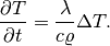
For the purpose of using Runge-Kutta methods, the equation has to be formulated in such a way that the time derivative stands solo on the left-hand side and everything else is on the right
(1)
Weak formulation
The temporal derivative is skipped, and weak formulation is only done for the right-hand side
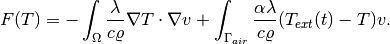
This approach is very different from the previous example P03/01-implicit-euler where the discretization of the time derivative term was hardwired into the weak formulation.
The function  above is the stationary residual of the equation (i.e., the weak form of the right-hand side).
Since the Runge-Kutta equations are solved using the Newton’s method, the reader may want to look at
the Newton’s method section in Part II before
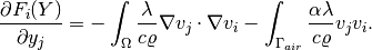
reading further. The weak form for the Jacobian matrix of the stationary residual is
above is the stationary residual of the equation (i.e., the weak form of the right-hand side).
Since the Runge-Kutta equations are solved using the Newton’s method, the reader may want to look at
the Newton’s method section in Part II before
reading further. The weak form for the Jacobian matrix of the stationary residual is
Defining weak forms
The weak forms are very similar to the previous example, except that the terms corresponding to the time derivative are missing, and the rest has an opposite sign (see files definitions.h and definitions.cpp).
Selecting a Butcher’s table
Unless the user wants to define a Butcher’s table on his/her own, he/she can select a predefined one - for example a second-order diagonally implicit SDIRK-22 method:
ButcherTableType butcher_table_type = Implicit_SDIRK_2_2;
This is followed in main.cpp by creating an instance of the table:
ButcherTable bt(butcher_table_type);
Initializing Runge-Kutta time stepping
This is done by instantiating the RungeKutta class. Passed are pointers to the discrete problem, Butcher’s table, and matrix solver:
// Initialize Runge-Kutta time stepping.
RungeKutta<double> runge_kutta(&wf, &space, &bt);


            // Some optional adjustments of default parameters
            runge_kutta.set_newton_tol(NEWTON_TOL);
            runge_kutta.set_newton_max_iter(NEWTON_MAX_ITER);
            runge_kutta.set_verbose_output(true);
            runge_kutta.set_newton_damping_coeff(1.0);
            runge_kutta.set_newton_max_allowed_residual_norm(1e10);
Time-stepping loop
The time-stepping loop has the form:
// Time stepping loop:
int ts = 1;
do
{
  // Perform one Runge-Kutta time step according to the selected Butcher's table.
  info("Runge-Kutta time step (t = %g s, time step = %g s, stages: %d).",
        current_time, time_step, bt.get_size());

              // This is important, these methods are shared by all the 'calculation' classes, i.e. RungeKutta, NewtonSolver, PicardSolver, LinearSolver,
                    DiscreteProblem, DiscreteProblemLinear.
              runge_kutta.setTime(current_time);
  runge_kutta.setTimeStep(time_step);

              try
  {
    runge_kutta.rk_time_step_newton(&sln_time_prev, &sln_time_new);
                    }
                    catch(std::exception& e)
  {
                            std::cout << e.what();
                            Hermes::Mixins::Loggable::Static::info("Runge-Kutta time step failed, try to decrease time step size.");
  }

  // Show the new time level solution.
  char title[100];
  sprintf(title, "Time %3.2f s", current_time);
  Tview.set_title(title);
  Tview.show(&sln_time_new);

  // Copy solution for the new time step.
  sln_time_prev.copy(&sln_time_new);

  // Increase current time and time step counter.
  current_time += time_step;
  ts++;
}
while (current_time < T_FINAL);