Systems of Equations (08-system)
So far we have solved single PDEs with a weak formulation
of the form  , where
  was a continuous approximation in the
 space. Hermes can also solve equations whose solutions lie in the spaces
 ,
,  or
or  , and one can combine these spaces for PDE systems
arbitrarily.
, and one can combine these spaces for PDE systems
arbitrarily.
General scheme
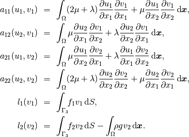
First let us understand how Hermes handles systems of linear PDE whose weak formulation is written as
(1)
The solution  and test functions
  belong to the space
  , where each
  is one of the available function spaces ,
, or . The resulting discrete matrix problem will have
an
is one of the available function spaces ,
, or . The resulting discrete matrix problem will have
an  block structure.
Model problem of linear elasticity
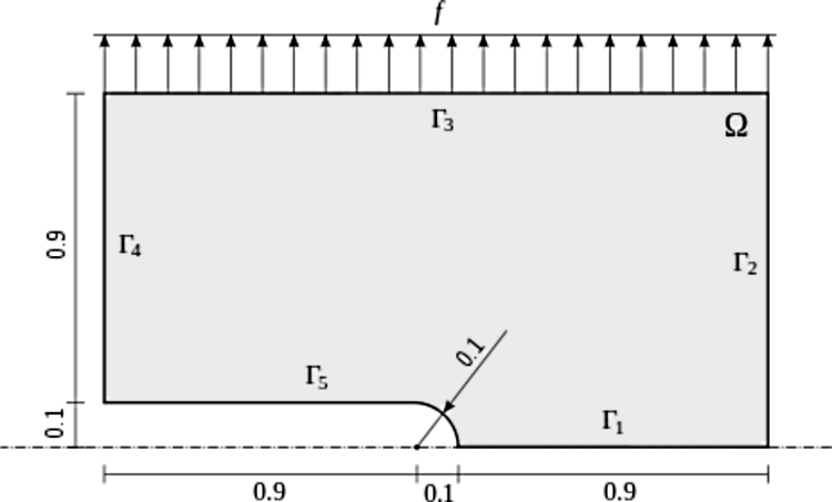
Let us illustrate this by solving a simple problem of linear elasticity. Consider a two-dimensional elastic body shown in the following figure. The lower edge has fixed displacements and the body is loaded with both an external force acting on the upper edge, and volumetric gravity force.
In the plane-strain model of linear elasticity the goal is to determine the
deformation of the elastic body. The deformation is sought as a vector
function  , describing the displacement of each point
 .
.
Boundary conditions
The boundary conditions are
The zero displacements are implemented as follows:
// Initialize boundary conditions.
DefaultEssentialBCConst<double> zero_disp("Bottom", 0.0);
EssentialBCs<double> bcs(&zero_disp);
The surface force is a Neumann boundary conditions that will be incorporated into the weak formulation.
Displacement spaces
Next we define function spaces for the two solution
components,  and
and  :
:
// Create x- and y- displacement space using the default H1 shapeset.
H1Space<double> u1_space(&mesh, &bcs, P_INIT);
H1Space<double> u2_space(&mesh, &bcs, P_INIT);
int ndof = Space<double>::get_num_dofs(Hermes::vector<Space<double> *>(&u1_space, &u2_space));
info("ndof = %d", ndof);
Weak formulation
Applying the standard procedure to the elastostatic equilibrium equations, we arrive at the following weak formulation:
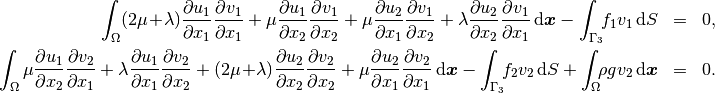
(the gravitational acceleration  is considered negative).
We see that the weak formulation can be written in the form (1):
is considered negative).
We see that the weak formulation can be written in the form (1):
Here,  and
and  are material constants (Lame coefficients) defined as
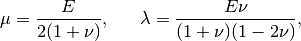
where  is the Young modulus and
  the Poisson ratio of the material. For
steel it is
the Poisson ratio of the material. For
steel it is  GPa and
  . The load force is
 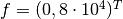 N.
N.
Definition of weak forms
Hermes provides default Jacobian and residual forms for linear elasticity (see Doxygen documentation). These are volumetric forms that can be used for problems with Dirichlet and/or zero Neumann boundary conditions. The weak formulation for this problem is implemented using those forms (see definitions.h and definitions.cpp).
In the forms, the block index  ,
,  means that the bilinear form takes basis functions from
space and test functions from space . I.e., the block index
0, 1 means that the bilinear form takes basis functions from space 0 (x-displacement space)
and test functions from space 1 (y-displacement space), etc. In this particular case the
Jacobian matrix has a
means that the bilinear form takes basis functions from
space and test functions from space . I.e., the block index
0, 1 means that the bilinear form takes basis functions from space 0 (x-displacement space)
and test functions from space 1 (y-displacement space), etc. In this particular case the
Jacobian matrix has a  block structure.
Flags HERMES_SYM, HERMES_NONSYM, HERMES_ANTISYM
Since the two diagonal forms  and
and  are symmetric, i.e.,
 , Hermes can be told to only evaluate half
of the integrals to speed up assembly. This is reflected by the parameter
HERMES_SYM in the constructors of these forms.
, Hermes can be told to only evaluate half
of the integrals to speed up assembly. This is reflected by the parameter
HERMES_SYM in the constructors of these forms.
The off-diagonal forms  and
and  are not
(and cannot) be symmetric, since their arguments come from different spaces in general.
However, we can see that
are not
(and cannot) be symmetric, since their arguments come from different spaces in general.
However, we can see that  , i.e., the corresponding blocks
of the local stiffness matrix are transposes of each other. Here, the HERMES_SYM flag
has a different effect: It tells Hermes to take the block of the local stiffness
matrix corresponding to the form
, i.e., the corresponding blocks
of the local stiffness matrix are transposes of each other. Here, the HERMES_SYM flag
has a different effect: It tells Hermes to take the block of the local stiffness
matrix corresponding to the form  , transpose it and copy it where a block
corresponding to
, transpose it and copy it where a block
corresponding to  belongs, without evaluating at all. This again
speeds up the matrix assembly. In other words, the form DefaultJacobianElasticity_1_0
is not needed.
belongs, without evaluating at all. This again
speeds up the matrix assembly. In other words, the form DefaultJacobianElasticity_1_0
is not needed.
Hermes also provides a flag HERMES_ANTISYM which is analogous to HERMES_SYM but the sign of the
copied block is changed. This flag is useful where  .
.
Even if your weak forms are symmetric, it is recommended to start with the default (and safe) flag HERMES_NONSYM. Once the model works, it can be optimized using the flag HERMES_SYM.
Assembling and solving the discrete problem using Newton’s method
When the spaces and weak forms are ready, one can initialize the Newton solver and adjust some parameters if necessary:
// Initialize Newton solver.
NewtonSolver<double> newton(&wf, Hermes::vector<Space<double> *>(&u1_space, &u2_space));
newton.set_verbose_output(true);
            newton.set_newton_tol(NEWTON_TOL);
            newton.set_newton_max_iter(NEWTON_MAX_ITER);
Next we perform the Newton’s iteration:
// Perform Newton's iteration.
try
{
  newton.solve();
}
catch(Hermes::Exceptions::Exception e)
{
  e.printMsg();
}
Note that two steps are taken although the problem is linear:
I ndof = 3000
I ---- Newton initial residual norm: 64400
I ---- Newton iter 1, residual norm: 4.52624e-07
I ---- Newton iter 2, residual norm: 9.7264e-09
<< close all views to continue >>
This confirms that using Newton for linear problems is useful. Last, the coefficient vector is translated into two displacement solutions:
// Translate the resulting coefficient vector into the Solution sln.
Solution<double> u1_sln, u2_sln;
Solution<double>::vector_to_solutions(newton.get_sln_vector(), Hermes::vector<const Space<double> *>(&u1_space, &u2_space),
    Hermes::vector<Solution<double> *>(&u1_sln, &u2_sln));
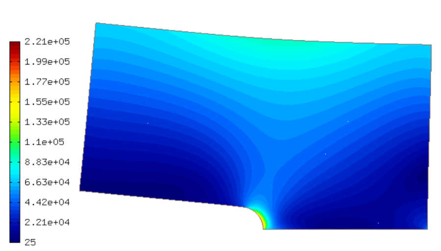
Visualizing the Von Mises stress
Hermes implements postprocessing through Filters. Filter is a special class which takes up to three Solutions, performs some computation and in the end acts as another Solution (which can be visualized, passed into another Filter, passed into a weak form, etc.). More advanced usage of Filters will be discussed later.
In elasticity examples we typically use the predefined VonMisesFilter:
// Visualize the solution.
ScalarView view("Von Mises stress [Pa]", new WinGeom(590, 0, 700, 400));
double lambda = (E * nu) / ((1 + nu) * (1 - 2*nu));  // First Lame constant.
double mu = E / (2*(1 + nu));                        // Second Lame constant.
VonMisesFilter stress(Hermes::vector<MeshFunction *>(&u1_sln, &u2_sln), lambda, mu);
view.show_mesh(false);
view.show(&stress, HERMES_EPS_HIGH, H2D_FN_VAL_0, &u1_sln, &u2_sln, 1.5e5);
Here the fourth and fifth parameters are the displacement components used to distort the domain geometry, and the sixth parameter is a scaling factor to multiply the displacements.