Axisymmetric Problems (09-axisym)
Model problem
We solve stationary heat transfer in a hollow cylindrical object shown in the following schematic picture:
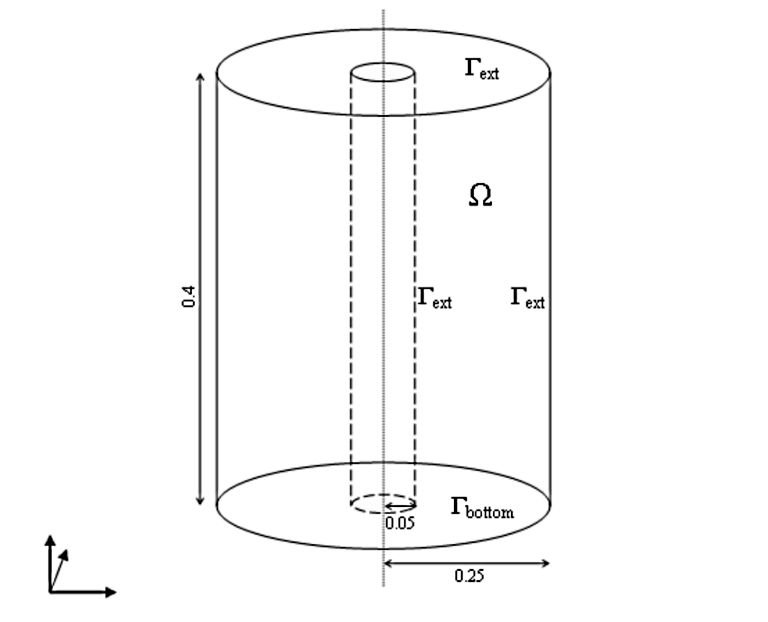
The symmetry axis of the object is aligned with the y-axis. The object stands on a hot plate

where  denotes its bottom face.
On the rest of the boundary we prescribe a radiation (Newton)
condition
denotes its bottom face.
On the rest of the boundary we prescribe a radiation (Newton)
condition
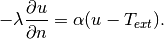
Here  is the
thermal conductivity of the material,
is the
thermal conductivity of the material,  the heat transfer
coefficient between the object and the air, and
the heat transfer
coefficient between the object and the air, and  the
exterior air temperature.
the
exterior air temperature.
Using default weak forms in axisymmetric mode
All default weak forms provided by Hermes can be used for 2D planar problems, 3D problems that are symmetric about the x-axis, and 3D problems that are symmetric about the y-axis. The mode is set via the optional parameter GeomType in the constructor of the default form. Thus the user can think in terms of the planar formulation of the problem, without having to bother with the axisymmetric forms of the differential operators.
The planar form of the stationary heat transfer equation is
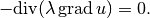
Hermes provides DefaultJacobianDiffusion and DefaultResidualDiffusion for the diffusion operator
For their headers we refer to the Doxygen documentation.
Custom weak forms
The weak formulation is custom because of the Newton boundary condition (see definitions.h and definitions.cpp).
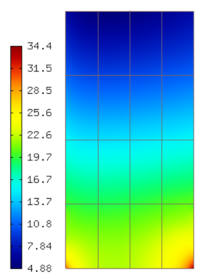
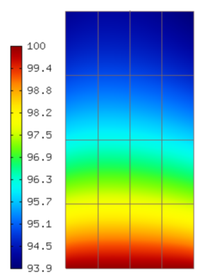
Sample results
Results for the values  ,
,  ,
,  and
and  are shown
below. We start with the stationary temperature distribution:
are shown
below. We start with the stationary temperature distribution:
and the following figure shows the temperature gradient: