General 2nd-Order Linear Equation (07-general)

The purpose of this example is threefold:

• To show how to define non-constant Dirichlet and Neumann boundary conditions.
• To illustrate how to handle spatially dependent equation coefficients.
• To introduce manual and automatic treatment of quadrature orders.

In particular the last item is worthwhile as numerical quadrature is one of the things that are very different in low-order and higher-order finite element methods.

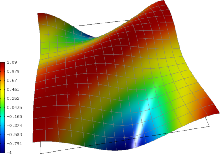
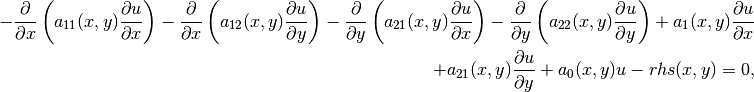
Model problem

We solve a linear second-order equation of the form

in a square domain . The equation is equipped with Dirichlet boundary conditions

on “Horizontal” boundary and with Neumann boundary conditions

on “Vertical” boundary.

Defining non-constant Dirichlet boundary conditions

Nonconstant Dirichlet boundary conditions are created by subclassing EssentialBoundaryCondition (see definitions.h):

class CustomEssentialBCNonConst : public EssentialBoundaryCondition<double>
{
public:
  CustomEssentialBCNonConst(std::string marker);

  inline EssentialBCValueType  get_value_type() const;

  virtual double value(double x, double y, double n_x, double n_y,
                       double t_x, double t_y) const;
};

The value returned will be a function, as opposed to a constant:

inline EssentialBoundaryCondition<double>::EssentialBCValueType CustomEssentialBCNonConst::get_value_type() const
{
  return EssentialBoundaryCondition<double>::BC_FUNCTION;
}

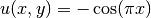
The value is defined using the virtual method value(). It can depend on the spatial coordinates as well as on the unit normal or tangential vectors to the boundary:

double CustomEssentialBCNonConst::value(double x, double y, double n_x, double n_y,
                                        double t_x, double t_y) const
{
  return -Hermes::cos(M_PI*x);
}

In both methods, be careful to use the “const” attribute - if you forget it, the compiler will complain that you have a purely virtual method in your new class.

Defining non-constant equation coefficients

The non-constant equation coefficients are defined here as global functions:

double a_11(double x, double y) { if (y > 0) return 1 + x*x + y*y; else return 1;}
double a_22(double x, double y) { if (y > 0) return 1; else return 1 + x*x + y*y;}
double a_12(double x, double y) { return 1; }
double a_21(double x, double y) { return 1;}
double a_1(double x, double y) { return 0.0;}
double a_2(double x, double y) { return 0.0;}
double a_0(double x, double y) { return 0.0;}

The custom weak formulation contains a volumetric matrix form, volumetric vector form, and a surface vector form that is due to the Neumann boundary conditions (see definitions.h and definitions.cpp).

Note that the method value() contains nonconstant coefficients defined by the user. Therefore, the user has to specify the quadrature order explicitly.

Setting the quadrature order manually

To do this, the user needs to redefine the purely virtual method ord():

Ord CustomWeakFormGeneral::MatrixFormVolGeneral::ord(int n, double *wt, Func<Ord> *u_ext[], Func<Ord> *u, Func<Ord> *v,
                                                     Geom<Ord> *e, ExtData<Ord> *ext) const
{
  // Returning the sum of the polynomial degrees of the basis and test function plus two.
  return u->val[0] * v->val[0] * e->x[0] * e->x[0];
}

This code does exactly what the comments says - the expression is parsed and the result of the analysis is a quadrature order Ord which equals to the sum of the polynomial degrees of the basis and test functions plus two. Quadrature orders in Hermes can be handled either automatically or manually. The above code is an example of the manual treatment that is needed since the coefficients and contain an “if-then” statement whose quadrature order is undefined.

If the expression contains any nonpolynomial function such as exp() or cos() then the parser automatically sets the quadrature order to 20, which can slow down the computation considerably. In situations like this, it may be better to handle the quadrature order manually.

Sample result

The output of this example is shown below: