Understanding Convergence Rates
Hermes provides convergence graphs for every adaptive computation. Therefore,
let us spend a short moment explaining their meaning.
The classical notion of  convergence rate is related to sequences of
uniform meshes with a gradually decreasing diameter h. In
convergence rate is related to sequences of
uniform meshes with a gradually decreasing diameter h. In  spatial dimensions,
the diameter h of a uniform mesh is related to the number of degrees of freedom
spatial dimensions,
the diameter h of a uniform mesh is related to the number of degrees of freedom  through the relation
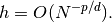
Therefore a slope of  on the log-log scale means that
 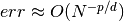 or
or  . When local refinements are enabled, the meaning of
convergence rate loses its meaning, and one should switch to convergence in terms of
the number of degrees of freedom (DOF) or CPU time - Hermes provides both.
. When local refinements are enabled, the meaning of
convergence rate loses its meaning, and one should switch to convergence in terms of
the number of degrees of freedom (DOF) or CPU time - Hermes provides both.
Algebraic convergence of adaptive h-FEM
When using elements of degree  , the convergence rate of adaptive h-FEM will not exceed the
one predicted for uniformly refined meshes (this can be explained using
mathematical analysis). Nevertheless, the convergence may be faster due to a different
constant in front of the
, the convergence rate of adaptive h-FEM will not exceed the
one predicted for uniformly refined meshes (this can be explained using
mathematical analysis). Nevertheless, the convergence may be faster due to a different
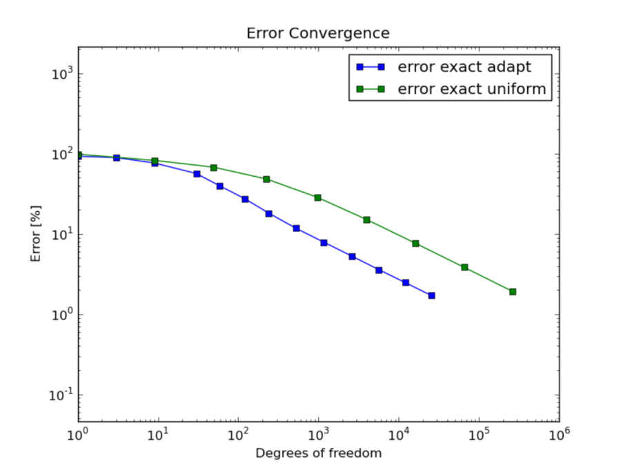
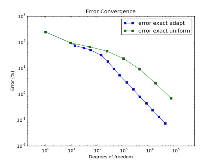
constant in front of the  term. This is illustrated in the following two figures,
both of which are related to a 2D problem with known exact solution. The first pair of
graphs corresponds to adaptive h-FEM with linear elements. The slope on the log-log
graph is -1/2 which means first-order convergence, as predicted by theory.
term. This is illustrated in the following two figures,
both of which are related to a 2D problem with known exact solution. The first pair of
graphs corresponds to adaptive h-FEM with linear elements. The slope on the log-log
graph is -1/2 which means first-order convergence, as predicted by theory.
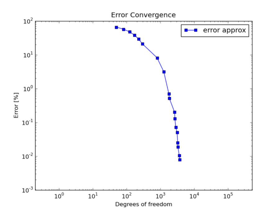
The next pair of convergence graphs corresponds to adaptive h-FEM with quadratic elements. The slope on the log-log graph is -1, which means that the convergence is quadratic as predicted by theory.
Note that one always should look at the end of the convergence curve, not at the beginning. The automatic adaptivity in Hermes is guided with the so-called reference solution, which is an approximation on a globally-refined mesh. In early stages of adaptivity, the reference solution and in turn also the error estimate usually are not sufficiently accurate to deliver the expected convergence rates.
Exponential convergence of adaptive hp-FEM
It is predicted by theory that adaptive hp-FEM should attain exponential convergence rate. This means that the slope of the convergence graph is the steeper the more one goes to the right:
While this is often the case with adaptive hp-FEM, there are problems whose difficulty is such that the convergence is not exponential. Or at least not during a long pre-asymptotic stage of adaptivity. This may happen, for example, when the solution contains an extremely strong singularity. Then basically all error is concentrated there, and all adaptive methods will do the same, which is to throw into the singularity as many small low-order elements as possible. Then the convergence of adaptive h-FEM and hp-FEM may be very similar (usually quite poor).
Estimated vs. exact convergence rates
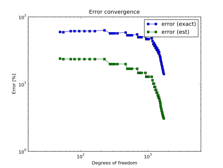
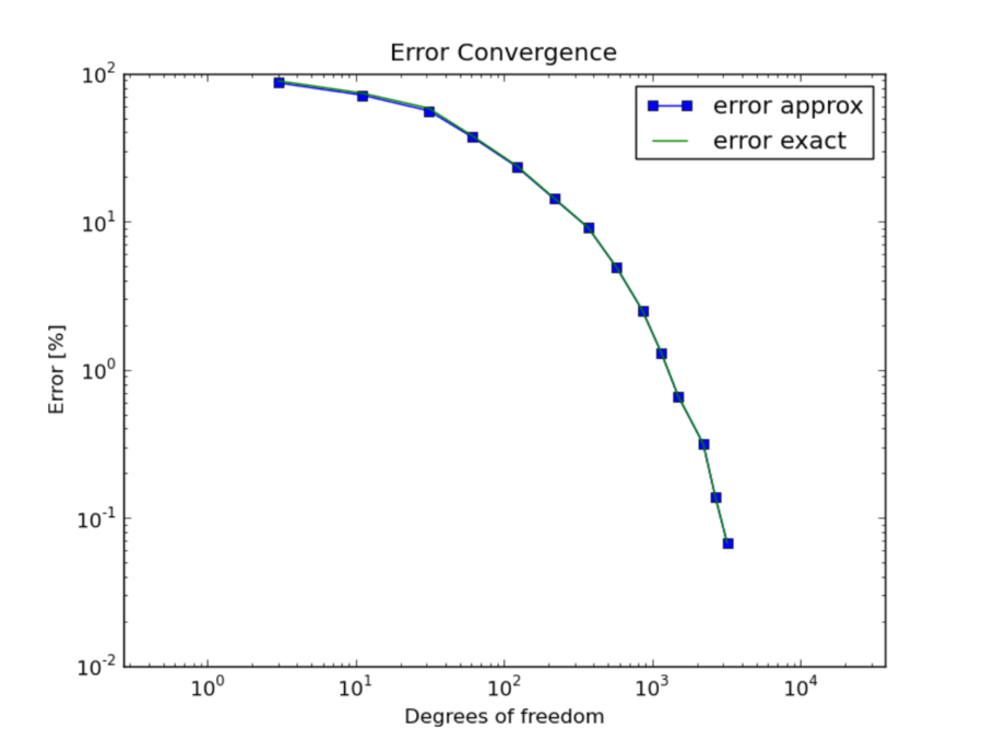
Whenever exact solution is available, Hermes provides both estimated error (via the reference solution) as well as the exact error. Thus the user can see the quality of the error estimate. Note that the estimated error usually is slightly less than the exact one, but during adaptivity they quickly converge together and become virtually identical. This is shown in the figure below.
In problems with extremely strong singularities the difference between the exact and estimated error can be significant. This is illustrated in the following graph that belongs to the benchmark “nist-10”.