Adaptive low-order FEM and hp-FEM

Our team has a passion for adaptive higher-order finite element methods because they are amazingly efficient compared to conventional low-order FEM. These methods have been an integral part of Hermes since its origin. Let us begin this tutorial chapter by explaining what gains the user can expect when using adaptive hp-FEM instead of conventional adaptive low-order FEM.

Low-order FEM is inefficient

Many practitioners are skeptical about using adaptive FEM because adaptivity can slow down and after some time virtually freeze a computation. The reason is that in conventional, algebraically-convergent FEM such as linear or quadratic, one needs to add more and more degrees of freedom to decrease the error. In fact the number of DOF needs to grow exponentially if the error is to decrease linearly. This phenomenon is problem-independent and it is due to poor approximation properties of low-order elements. In contrast to this, adaptive hp-FEM achieves linear decrease of error by adding degrees of freedom linearly. The different convergence rates of adaptive FEM with linear and quadratic elements, and adaptive hp-FEM is shown below. Note that on the log-log scale, the slope of the convergence curve tells the convergence rate of the method. If the slope is constant then the method converges algebraically.

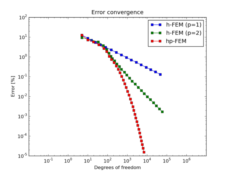
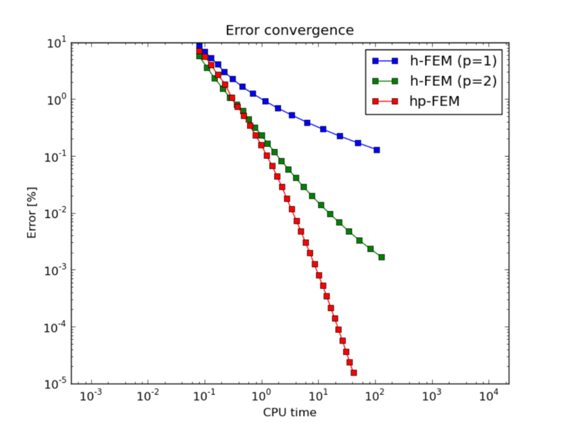
The reader can see that the linear FEM would need in the order of 1,000,000,000,000,000,000 degrees of freedom (DOF) to reach a level of accuracy where the hp-FEM is with less than 10,000 DOF. A similar effect can be observed in the CPU-time convergence graph:

These convergence curves are typical representative examples, confirmed with many numerical experiments of independent researchers, and supported with theory. Let us mention again that adaptive low-order FEM is doomed by the underlying math – its poor convergence cannot be fixed by designing smarter adaptivity algorithms.

What makes adaptive hp-FEM so fast

In order to obtain fast, usable adaptivity (represented by the red curve above), one has to resort to adaptive hp-FEM. The hp-FEM takes advantage of the following facts:

• Large high-order elements approximate smooth parts of the solution much more efficiently than small linear ones. An adaptive algorithm should use p-refinements (increase the polynomial degree of elements without subdividing them in space).
• This holds the other way round for singularities, steep gradients, oscillations and other “bad” features: These are approximated best using small low-order elements. In areas like this, the adaptive algorithm should use hp-refinements (subdivide elements in space and distribute polynomial degrees in the element sons in an optimal way).
• In order to capture efficiently anisotropic solution behavior such as boundary or internal layers, the adaptive algorithm should be able to refine the meshes anisotropically both in h and p. This is illustrated in several benchmarks including “smooth-aniso-x” and “nist-07”.

Benchmarks are part of the repository “hermes-examples” and we highly recommend the reader to check them out.

What does it take to do adaptive hp-FEM

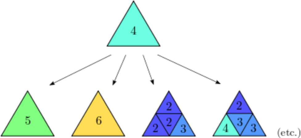
Automatic adaptivity in the hp-FEM is substantially different from adaptivity in low-order FEM, since every element can be refined in many different ways. The following figure shows several illustrative refinement candidates for a fourth-order element.

The number of allowed element refinements is implementation-dependent, but in general it is very low in h or p adaptivity, much higher in hp-adaptivity, and it rises even more when quadrilateral elements are used and their anisotropic refinements are enabled.

Eight hp-adaptivity modes in Hermes

Hermes has eight different adaptivity modes P_ISO, P_ANISO, H_ISO, H_ANISO, HP_ISO, HP_ANISO_P, HP_ANISO_H, HP_ANISO. In this order, usually P_ISO yields the worst results and HP_ANISO the best. However, even P_ISO can be very efficient with a good a-priori locally refined starting mesh.

The most general mode HP_ANISO considers around 100 refinement candidates for each element. The difference between the next best mode HP_ANISO_H and HP_ANISO is only significant for problems that exhibit strong anisotropic behavior. The selection of the hp-refinement mode is where the user can use his a-priori knowledge of the problem to make the computation faster.

Error estimate based on solution pair

Due to the large number of refinement options in each element, classical error estimators that provide just one number per element are not enough to guide hp-adaptivity. For that one needs to know the actual shape of the approximation error, not only its magnitude.

In analogy to the most successful adaptive ODE solvers, Hermes uses a pair of approximations with different orders of accuracy to obtain this information:

• Fine mesh solution.
• Its orthogonal projection on a coarse submesh.

The initial coarse submesh mesh is read from the mesh file, and the initial fine mesh is created through its global refinement both in h and p. The fine mesh solution is the approximation of interest both during the adaptive process and at the end of computation.

Robustness of the solution-pair approach

The solution-pair approach is PDE independent, which is truly invaluable for various types of single-physics problems and for multi-physics coupled problems. Hermes does not use a single analytical error estimate or any other technique that would narrow down its applicability to some selected class of equations.