An Introductory Example (01-intro)

Model problem

Let us demonstrate the use of adaptive h-FEM and hp-FEM on a linear elliptic problem describing an electrostatic micromotor. This is a MEMS device free of any coils, and thus (as opposed to classical electromotors) resistive to strong electromagnetic waves.

The following figure shows a symmetric half of the domain (dimensions need to be scaled with and they are in meters):

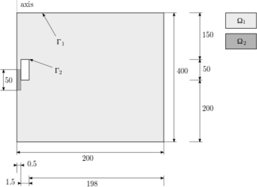
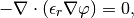
The subdomain represents the moving part of the domain and the area bounded by represents the electrodes that are fixed. The distribution of the electrostatic potential is governed by the equation

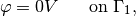
equipped with the Dirichlet boundary conditions

The relative permittivity is piecewise-constant, in and in .

Weak formulation

The weak forms are custom because of two materials are involved, see the files definitions.h and definitions.cpp.

Refinement selector

Before the adaptivity loop starts, a refinement selector is initialized:

// Initialize refinement selector.
H1ProjBasedSelector<double> selector(CAND_LIST, CONV_EXP, H2DRS_DEFAULT_ORDER);

The selector is used by the class Adapt to determine how an element should be refined. For that purpose, the selector does the following:

1. It generates candidates (proposed element refinements).
2. It estimates their local errors by projecting the reference solution onto their FE spaces.
3. It calculates the number of degree of freedom (DOF) contributed by each candidate.
4. It calculates a score for each candidate, and sorts them according to their scores.
5. It selects a candidate with the highest score. If the next candidate has almost the same score and symmetric mesh is preferred, it skips both of them. More detailed explanation of this will follow.

Score of refinement candidates

By default, the score is

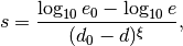
where and are an estimated error and an estimated number of DOF of a candidate respectively, and are an estimated error and an estimated number of DOF of the examined element respectively, and is a convergence exponent.

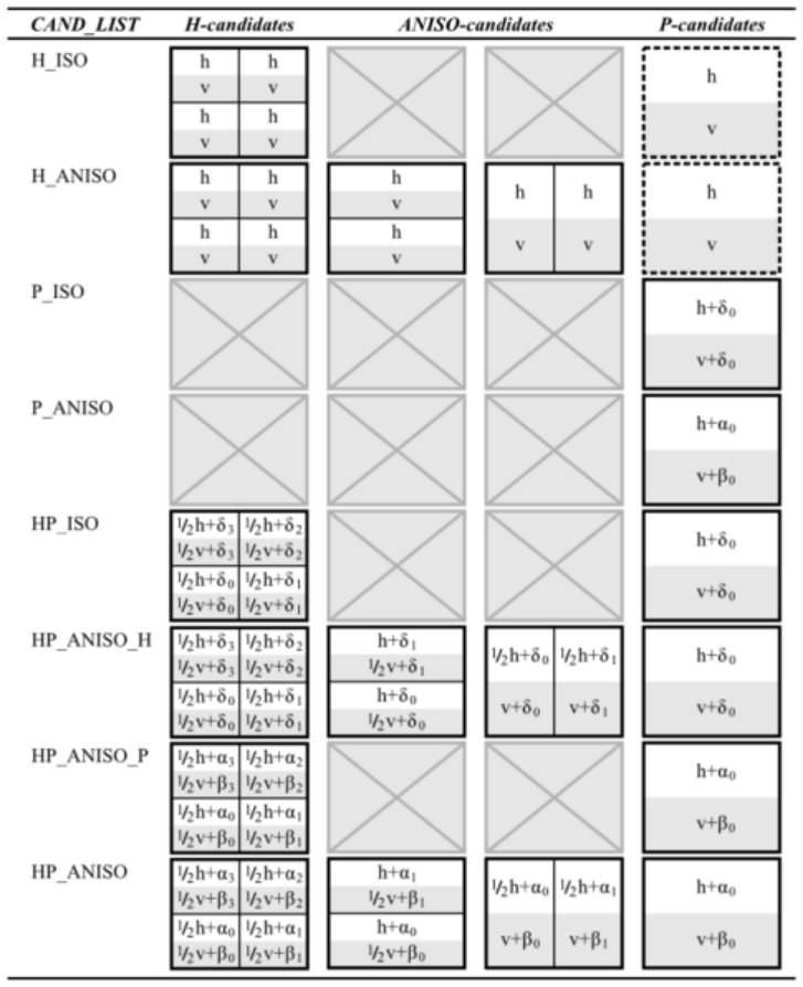
The first parameter CAND_LIST specifies which candidates are generated. In a case of quadrilaterals, all possible values and considered candidates are summarized in the following table:

The second parameter CONV_EXP is a convergence exponent used to calculate the score.

The third parameter specifies the the maximum considered order used in the resulting refinement. In this case, a constant H2DRS_DEFAULT_ORDER is used. The constant is defined by Hermes2D library and it corresponds to the maximum order supported by the selector. In this case it is 9.

Weighting refinement candidates

Furthermore, the selector allows you to weight errors though a method set_error_weights(). Error weights are applied before the error of a candidate is passed to the calculation of the score. Through this method it is possible to set a preference for a given type of a candidate, i.e., H-candidate, P-candidate, and ANISO-candidate. The error weights can be set anytime and setting error weights to appropriate values can lead to a lower number of DOF. However, the best values of weights depend on a solved problem.

In this particular case, a default error weights are used. The default weights prefer the P-candidate and they are defined as:

• H-candidate weight: (see a constant H2DRS_DEFAULT_ERR_WEIGHT_H)
• P-candidate weight: (see a constant H2DRS_DEFAULT_ERR_WEIGHT_P)
• ANISO-candidate weight: (see a constant H2DRS_DEFAULT_ERR_WEIGHT_ANISO)

Since these weights are default, it is not necessary to express them explicitly. Nevertheless, if expressed, a particular line of the code would be:

selector.set_error_weights(2.0, 1.0, sqrt(2.0));

Modifying default behavior

Besides the error weights, the selector allows you to modify a default behaviour through the method set_option(). The behavior can be modified anytime. Currently, the method accepts following options:

• H2D_PREFER_SYMMETRIC_MESH: Prefer symmetric mesh when selection of the best candidate is done. If set and if two or more candidates has the same score, they are skipped. This option is set by default.
• H2D_APPLY_CONV_EXP_DOF: Use , where is the convergence exponent, instead of to evaluate the score. This options is not set by default.

In this case, default settings are used. If expressed explicitly, the code would be:

selector.set_option(H2D_PREFER_SYMMETRIC_MESH, true);
selector.set_option(H2D_APPLY_CONV_EXP_DOF, false);

Plotting convergence graphs

In order to plot convergence graphs, one can use the SimpleGraph class:

// DOF and CPU convergence graphs.
SimpleGraph graph_dof_est, graph_cpu_est;

This class will save convergence data as two numbers per line: either the number of DOF and error, or CPU time and error. A more advanced GnuplotGraph class is also available.

Adaptivity loop

The adaptivity algorithm in Hermes calculates an approximation on fine mesh and uses orthogonal projection to a coarse submesh to extract low-order part of the solution. This gives two approximations with different orders of accuracy whose difference is used as an a-posteriori error estimate (error function). The error function is used to decide which elements need to be refined as well as to select optimal hp-refinement for each element. Hence the adaptivity loop begins with refining the mesh globally:

// Construct globally refined mesh and setup fine mesh space.
Space<double>* ref_space = Space<double>::construct_refined_space(&space);

The new spaces have to be set to the Newton solver that we already created (outside of the adaptivity loop):

newton.set_space(ref_space);

The Newton’s method is used to solve the fine mesh problem:

// Perform Newton's iteration.
try
{
  newton.solve(coeff_vec);
}
catch(Hermes::Exceptions::Exception e)
{
  e.printMsg();

}

The coefficient vector is translated into a Solution. The pointer(s) to Space(s) needs to be constant, but we omit that here for simplicity:

// Translate the resulting coefficient vector into the instance of Solution.
Solution<double>::vector_to_solution(newton.get_sln_vector(), ref_space, &ref_sln);

The Solution is projected on the coarse submesh to extract low-order part for error calculation:

// Project the fine mesh solution onto the coarse mesh.
info("Projecting fine mesh solution on coarse mesh.");
OGProjection<double> ogProjection; ogProjection.project_global(&space, &ref_sln, &sln);

The function project_global() is very general, and it can accept multiple spaces, multiple functions, and various projection norms as parameters. For more details, see Doxygen documentation.

Calculating error estimate

The coarse and reference mesh approximations are inserted into the class Adapt and a global error estimate as well as element error estimates are calculated:

info("Calculating error estimate.");
Adapt<double> adaptivity(&space);
bool solutions_for_adapt = true;
double err_est_rel = adaptivity.calc_err_est(&sln, &ref_sln, solutions_for_adapt,
                     HERMES_TOTAL_ERROR_REL | HERMES_ELEMENT_ERROR_REL) * 100;

Here, solutions_for_adapt=true means that this solution pair will be used to calculate element errors to guide adaptivity. With solutions_for_adapt=false, just the total error would be calculated (not the element errors).

When working with another space than , the HERMES_H1_NORM can be replaced with HERMES_HCURL_NORM, HERMES_HDIV_NORM, or HERMES_L2_NORM. For equation systems, a Hermes::vector<int> with multiple norms can be used.

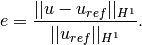
The error estimate is calculated as

Adapting the mesh

Finally, if err_est_rel is still above the threshold ERR_STOP, we perform mesh adaptation:

// Skip the time spent to save the convergence graphs.
cpu_time.tick(HERMES_SKIP);

// If err_est too large, adapt the mesh.
if (err_est_rel < ERR_STOP)
  done = true;
else
{
  info("Adapting coarse mesh.");
  done = adaptivity.adapt(&selector, THRESHOLD, STRATEGY, MESH_REGULARITY);

  // Increase the counter of performed adaptivity steps.
  if (done == false)
    as++;
}
if (space.get_num_dofs() >= NDOF_STOP)
  done = true;

The constants THRESHOLD, STRATEGY and MESH_REGULARITY have the following meaning:

Adaptive strategies

The constant STRATEGY indicates which adaptive strategy is used. In all cases, the strategy is applied to elements in an order defined through the error. If the user request to process an element outside this order, the element is processed regardless the strategy. Currently, Hermes2D supportes following strategies:

• STRATEGY == 0: Refine elements until sqrt(THRESHOLD) times total error is processed. If more elements have similar error refine all to keep the mesh symmetric.
• STRATEGY == 1: Refine all elements whose error is bigger than THRESHOLD times the error of the first processed element, i.e., the maximum error of an element.
• STRATEGY == 2: Refine all elements whose error is bigger than THRESHOLD.

Mesh regularity

The constant MESH_REGULARITY specifies maximum allowed level of hanging nodes: -1 means arbitrary-level hanging nodes (default), and 1, 2, 3, ... means 1-irregular mesh, 2-irregular mesh, etc. Hermes does not support adaptivity on regular meshes because of its extremely poor performance.

It is a good idea to spend some time playing with these parameters to get a feeling for adaptive hp-FEM. Also look at other adaptivity examples in the examples/ directory: layer, lshape deal with elliptic problems and have known exact solutions. So do examples screen, bessel for time-harmonic Maxwell’s equations. These examples allow you to compare the error estimates computed by Hermes with the true error. Examples crack, singpert show how to handle cracks and singularly perturbed problems, respectively. There are also more advanced examples illustrating automatic adaptivity for nonlinear problems solved via the Newton’s method, adaptive multimesh hp-FEM, adaptivity for time-dependent problems on dynamical meshes, etc.

Sample results

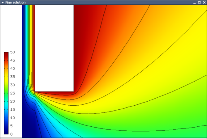
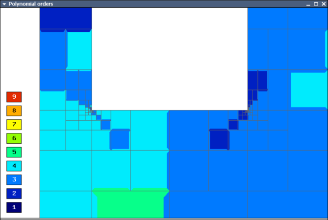
The computation starts with a very coarse mesh consisting of a few quadrilaterals, some of which are moreover very ill-shaped. Thanks to the anisotropic refinement capabilities of the selector, the mesh quickly adapts to the solution and elements of reasonable shape are created near singularities, which occur at the corners of the electrode. Initially, all elements of the mesh are of a low degree, but as the hp-adaptive process progresses, the elements receive different polynomial degrees, depending on the local smoothness of the solution.

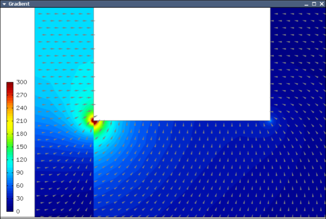
The gradient was visualized using the class VectorView. We have seen this in the previous section. We plug in the same solution for both vector components, but specify that its derivatives should be used:

gview.show(&sln, &sln, H2D_EPS_NORMAL, H2D_FN_DX_0, H2D_FN_DY_0);

---

---

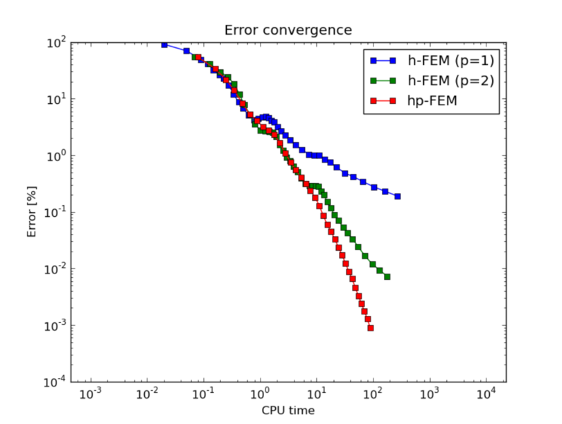
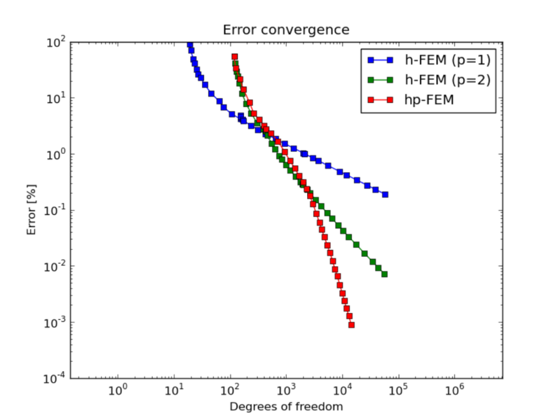
Convergence graphs of adaptive h-FEM with linear elements, h-FEM with quadratic elements and hp-FEM are shown below.

The following graph shows convergence in terms of CPU time.