Transient Problems II - Adaptivity in Time (09-transient-time-only)

Model problem

This example is analogous to example “P04-adaptivity/07-transient-space-only” except that a fixed mesh is used and only the time stepping is adaptive. An arbitrary embedded Runge-Kutta method can be used. By embedded we mean that the Butcher’s table contains two B rows. The two B rows are used to calculate two different approximations on the next time level, with different orders of accuracy. The difference between these two solutions is used as an error estimate, to adapt the time step.

Selecting an embedded Runge-Kutta method

Hermes provides by default the following embedded explicit methods:

• Explicit_HEUN_EULER_2_12_embedded,
• Explicit_BOGACKI_SHAMPINE_4_23_embedded,
• Explicit_FEHLBERG_6_45_embedded,
• Explicit_CASH_KARP_6_45_embedded,
• Explicit_DORMAND_PRINCE_7_45_embedded,

and the following embedded implicit methods:

• Implicit_SDIRK_CASH_3_23_embedded,
• Implicit_ESDIRK_TRBDF2_3_23_embedded,
• Implicit_ESDIRK_TRX2_3_23_embedded,
• Implicit_SDIRK_BILLINGTON_3_23_embedded,
• Implicit_SDIRK_CASH_5_24_embedded,
• Implicit_SDIRK_CASH_5_34_embedded,
• Implicit_DIRK_ISMAIL_7_45_embedded.

We usually use the SDIRK methods by Cash as they work really well.

Obtaining temporal error estimate

When the Butcher’s table is an embedded one, the method rk_time_step_newton() provides an error estimate on the next time level (difference of the two approximations with different orders of accuracy):

// Perform one Runge-Kutta time step according to the selected Butcher's table.
info("Runge-Kutta time step (t = %g, tau = %g, stages: %d).",
     current_time, time_step, bt.get_size());

            runge_kutta.setTime(current_time);
            runge_kutta.setTimeStep(time_step);

            try
            {
                    runge_kutta.rk_time_step_newton(&sln_time_prev, &sln_time_new);
            }
catch(Exceptions::Exception& e)
{
  e.printMsg();
}

The solution sln_time_new contains the more accurate of the two solutions.

Calculating relative temporal error

This is done by calculating the norm of the error function and dividing it by the norm of the solution:

double rel_err_time = Global<double>::calc_norm(&time_error_fn, HERMES_H1_NORM) /
                      Global<double>::calc_norm(&sln_time_new, HERMES_H1_NORM) * 100;

Adapting the time step

There are many ways to do this, let us show a very simple one here. We define two tolerances for the relative temporal error: TIME_TOL_UPPER and TIME_TOL_LOWER. If the time step exceeds the former, then the time step is decreased and vice versa. The code is very simple:

if (rel_err_time > TIME_TOL_UPPER) {
  info("rel_err_time above upper limit %g%% -> decreasing time step from %g to %g and repeating time step.",
       TIME_TOL_UPPER, time_step, time_step * TIME_STEP_DEC_RATIO);
  time_step *= TIME_STEP_DEC_RATIO;
  continue;
}
if (rel_err_time < TIME_TOL_LOWER) {
  info("rel_err_time = below lower limit %g%% -> increasing time step from %g to %g",
       TIME_TOL_UPPER, time_step, time_step * TIME_STEP_INC_RATIO);
  time_step *= TIME_STEP_INC_RATIO;
}

Plotting the temporal error estimate

The temporal error is a function that is usually positive in some parts of the computational domain and negative elsewhere. As the magnitude is what matters, it may be a good idea to use an AbsFilter:

// Plot error function.
char title[100];
sprintf(title, "Temporal error, t = %g", current_time);
eview.set_title(title);
AbsFilter abs_tef(&time_error_fn);
eview.show(&abs_tef);

Here, the option HERMES_EPS_VERYHIGH is used to render accurately a function that has very small values.

Sample results

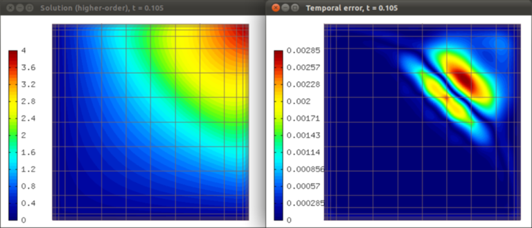
Solution and temporal error at t = 0.105 s:

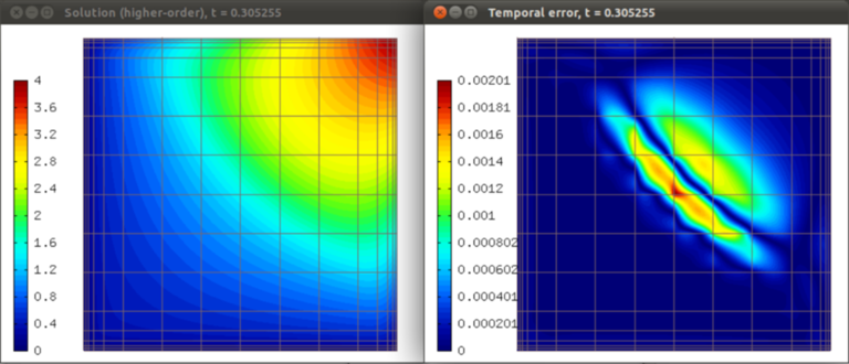
Solution and temporal error at t = 0.305 s:

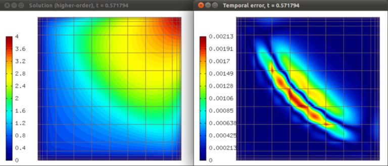
Solution and temporal error at t = 0.572 s:

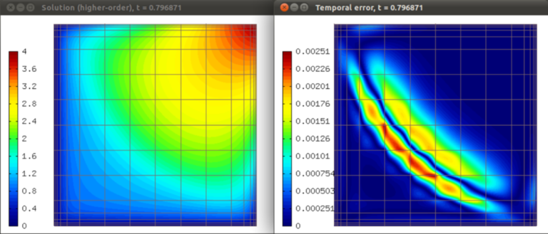
Solution and temporal error at t = 0.797 s:

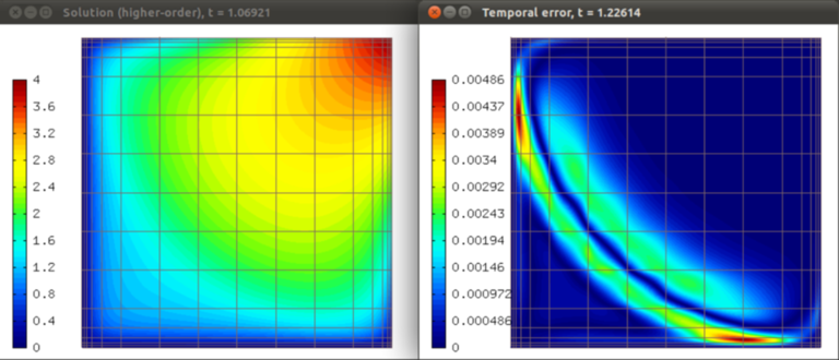
Solution and temporal error at t = 1.226 s: