Transient Problems I - Adaptivity in Space (08-transient-space-only)
Model problem
This example is derived from example “P03-timedep/03-nonlinear” and it shows how automatic adaptivity in space can be combined with arbitrary Runge-Kutta methods in time. The example uses fixed time step size.
We consider a nonlinear time-dependent equation of the form
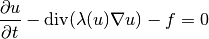
equipped with Dirichlet boundary conditions and solved in a square domain
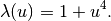
 . The nonlinearity
  has the form
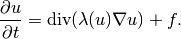
Recall that for the Runge-Kutta methods, we need the time derivative on the left and everything else on the right,
Weak forms are created for the right-hand side only and we have seen them before.
Time stepping and periodic mesh derefinement
Mesh derefinement is necessary in adaptive FEM for time-dependent problems, and it is much more complicated than mesh refinement. This is because one cannot spoil much by doing a wrong mesh refinement, but a wrong mesh derefinement can cause lots of damage.
There are three ways to perform global mesh derefinement in Hermes:
- Reset the mesh to basemesh and reset polynomial orders to P_INIT.
- Remove last layer of refinement from all elements, and reset polynomial orders to P_INIT.
- Remove last layer of refinement from all elements, and decrease polynomial orders by one.
The derefinement frequency is set by the user via the parameter UNREF_FREQ:
// Periodic global derefinement.
if (ts > 1 && ts % UNREF_FREQ == 0)
{
  info("Global mesh derefinement.");
  switch (UNREF_METHOD) {
    case 1: mesh.copy(&basemesh);
            space.set_uniform_order(P_INIT);
            break;
    case 2: mesh.unrefine_all_elements();
            space.set_uniform_order(P_INIT);
            break;
    case 3: mesh.unrefine_all_elements();
            //space.adjust_element_order(-1, P_INIT);
            space.adjust_element_order(-1, -1, P_INIT, P_INIT);
            break;
    default: error("Wrong global derefinement method.");
  }

  ndof_coarse = Space<double>::get_num_dofs(&space);
}
Option #1 is cleanest from the mathematics point of view since the mesh on the new time level will not be influenced by the mesh from the last step, but in practice we prefer the last option because it takes less CPU time.
The adaptivity loop in space is standard. The rk_time_step_newton() method is called in each adaptivity step:
// Perform one Runge-Kutta time step according to the selected Butcher's table.
info("Runge-Kutta time step (t = %g s, tau = %g s, stages: %d).",
     current_time, time_step, bt.get_size());

                  runge_kutta.setTime(current_time);
                  runge_kutta.setTimeStep(time_step);

try
{
  runge_kutta.rk_time_step_newton(&sln_time_prev, &sln_time_new);
}
catch(Exceptions::Exception& e)
{
  e.printMsg();

}
The value of current_time and the previous time level solution sln_time_prev do not change during spatial adaptivity.
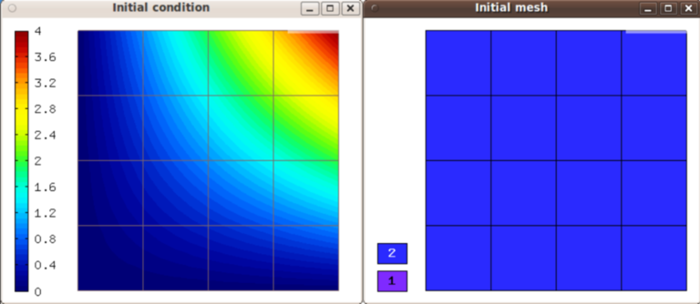
Sample results
Initial condition and initial mesh:
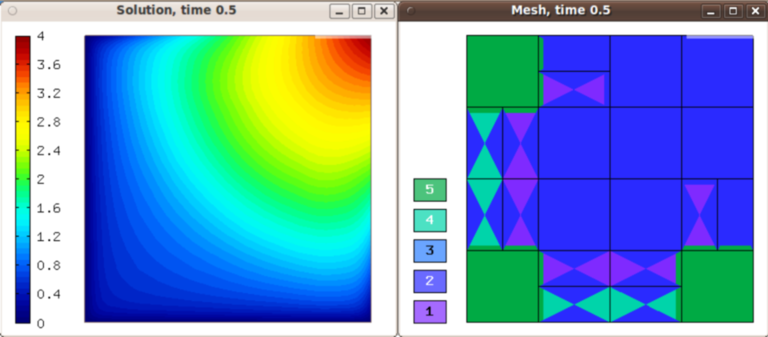
Solution and mesh at t = 0.5:
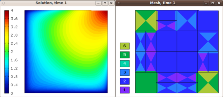
Solution and mesh at t = 1.0:
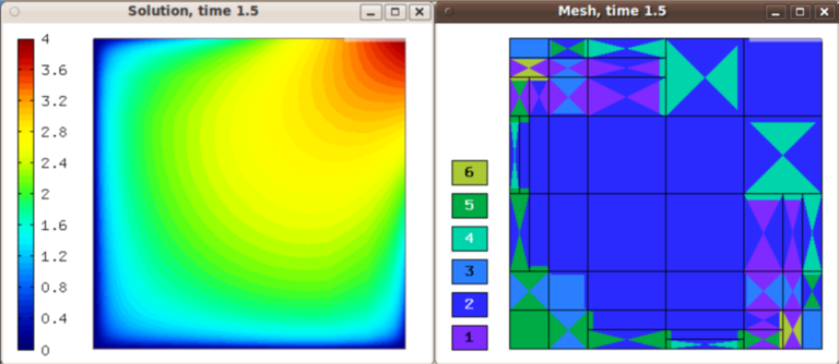
Solution and mesh at t = 1.5:
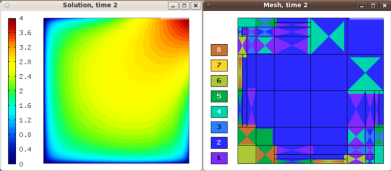
Solution and mesh at t = 2.0: