Newton’s Method with Analytic Nonlinearity (02-newton-analytic)

Model problem

We will keep the model problem from the previous sections,

Recall that the domain is a square 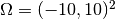, , and the nonlinearity has the form

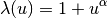
where is an even nonnegative integer. Also recall from the previous section that

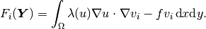
and

Initializing the weak formulation

This is very simple, using the predefined DefaultWeakFormPoisson class:

// Initialize the weak formulation
CustomNonlinearity lambda(alpha);
Hermes2DFunction<double> src(-heat_src);
DefaultWeakFormPoisson<double> wf(HERMES_ANY, &lambda, &src);

We should mention that the CustomNonlinearity class is identical with example 01-picard.

Obtaining a good initial coefficient vector

It is possible to start the Newton’s method from the zero vector, but then the convergence may be slow or the method may diverge. We usually prefer to project an initial solution guess (a function) on the finite element space, to obtain an initial coefficient vector:

// Project the initial condition on the FE space to obtain initial
// coefficient vector for the Newton's method.
// NOTE: If you want to start from the zero vector, just define
// coeff_vec to be a vector of ndof zeros (no projection is needed).
info("Projecting to obtain initial vector for the Newton's method.");
double* coeff_vec = new double[ndof];
CustomInitialCondition init_sln(&mesh);
OGProjection<double> ogProjection; ogProjection.project_global(&space, &init_sln, coeff_vec);

The Newton’s iteration loop

The Newton’s iteration loop is done as in linear problems:

// Initialize Newton solver.
NewtonSolver<double> newton(&dp);

// Perform Newton's iteration.
try
{
  newton.solve(coeff_vec);
}
catch(Hermes::Exceptions::Exception e)
{
  e.printMsg();
}

Note that the Newton’s loop always handles a coefficient vector, not Solutions.

Translating the resulting coefficient vector into a Solution

After the Newton’s loop is finished, the resulting coefficient vector is translated into a Solution as follows:

// Translate the resulting coefficient vector into a Solution.
Solution<double> sln;
Solution<double>::vector_to_solution(newton.get_sln_vector(), &space, &sln);

Cleaning up

As a last step, we clean up as usual:

// Clean up.
delete [] coeff_vec;

Convergence

Compare the following with the convergence of the Picard’s method in example 01-picard:

I ndof: 961
I Projecting to obtain initial vector for the Newton's method.
I ---- Newton initial residual norm: 1160.42
I ---- Newton iter 1, residual norm: 949.355
I ---- Newton iter 2, residual norm: 291.984
I ---- Newton iter 3, residual norm: 78.189
I ---- Newton iter 4, residual norm: 13.0967
I ---- Newton iter 5, residual norm: 0.585997
I ---- Newton iter 6, residual norm: 0.00127226
I ---- Newton iter 7, residual norm: 5.27303e-09
  << close all views to continue >>

Sample results

The resulting approximation is the same as in example P02/01-picard.