Introduction to Newton’s Method
The Newton’s method is more powerful but also a bit more demanding than the Picard’s method.
We’ll stay with the model problem from the previous section
(1)
As we said before, when using the Newton’s method, it is customary to have everything on the left-hand side. The corresponding discrete problem has the form

where  are the test functions. The unknown solution
  is sought in the form
where  is a Dirichlet lift (any sufficiently smooth function representing the
Dirichlet boundary conditions
is a Dirichlet lift (any sufficiently smooth function representing the
Dirichlet boundary conditions  ), and
  with zero values on the boundary is
a new unknown. The function
with zero values on the boundary is
a new unknown. The function  is expressed as a linear combination of basis functions
with unknown coefficients,
is expressed as a linear combination of basis functions
with unknown coefficients,
However, in the Newton’s method we look at the same function
as at a function of the unknown solution coefficient vector  ,
,
The nonlinear discrete problem can be written in a compact form

where 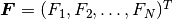 is the so-called residuum or residual vector.
Residual vector and Jacobian matrix
The residual vector  has
has  components of the form
Here is the  -th test function,
 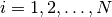 .
The
.
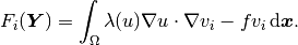
The  Jacobian matrix
 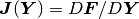 has the components
![J_{ij}(\bfY) = \frac{\partial F_i}{\partial y_j} =
\int_{\Omega} \left[ \frac{\partial \lambda}{\partial u} \frac{\partial u}{\partial y_j}
\nabla u + \lambda(u)\frac{\partial \nabla u}{\partial y_j} \right] \cdot \nabla v_i \, \mbox{d}\bfx.](../../../_images/math/d410d28c4aacc645798c1ec5ef11467e4e388748.png)
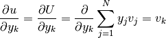
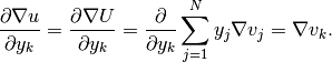
Taking account the relation  , and the independence of
  on
on  , this becomes
![J_{ij}(\bfY) = \frac{\partial F_i}{\partial y_j} =
\int_{\Omega} \left[ \frac{\partial \lambda}{\partial u} \frac{\partial U}{\partial y_j}
\nabla u + \lambda(u)\frac{\partial \nabla U}{\partial y_j} \right] \cdot \nabla v_i \, \mbox{d}\bfx.](../../../_images/math/67f9f9640d27371567ce1a31f287ad964a592143.png)
Using elementary relations shown below, we obtain
![J_{ij}(\bfY) =
\int_{\Omega} \left[ \frac{\partial \lambda}{\partial u}(u) v_j
\nabla u + \lambda(u)\nabla v_j \right] \cdot \nabla v_i \, \mbox{d}\bfx.](../../../_images/math/3b81b579f3778c8f02c7c1098fce38adb35cc3e5.png)
It is worth noticing that  has the same sparsity structure as the
standard stiffness matrix that we know from linear problems. In fact, when the
problem is linear then the Jacobian matrix and the stiffness matrix are the same
thing – we have seen this before, and also see the last paragraph in this section.
has the same sparsity structure as the
standard stiffness matrix that we know from linear problems. In fact, when the
problem is linear then the Jacobian matrix and the stiffness matrix are the same
thing – we have seen this before, and also see the last paragraph in this section.
How to differentiate weak forms
Chain rule is used all the time. If your equation contains parameters that depend on
the solution, you will need their derivatives with respect to the solution (such as we needed
the derivative  above). In addition, the following elementary rules are useful
for the differentiation of the weak forms:
above). In addition, the following elementary rules are useful
for the differentiation of the weak forms:
and
Practical formula
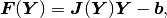
Let’s assume that the Jacobian matrix has been assembled. The Newton’s method is written formally as

but a more practical formula to work with is

This is a system of linear algebraic equations that needs to be solved in every Newton’s
iteration. The Newton’s method will stop when  is sufficiently close
to the zero vector.
is sufficiently close
to the zero vector.
Stopping criteria
There are two basic stopping criteria that should be combined for safety:
- Checking whether the (Euclidean) norm of the residual vector
 is sufficiently close to zero.
 - Checking whether the norm of
 is sufficiently close to zero.
If just one of these two criteria is used, the Newton’s method may finish prematurely.
Linear problems
In the linear case we have
where  is a constant stiffness matrix and
  a load vector.
The Newton’s method is now
a load vector.
The Newton’s method is now

There exists a widely adopted mistake saying that the Newton’s method, when applied to a linear problem, will converge in one iteration. This is only true if one uses the first (residual norm based) stopping criterion above. If the second criterion is used, which is based on the distance of two consecutive solution vectors, then the Newton’s method will do two steps before stopping. In practice, using just the residual criterion is dangerous.