Time-Harmonic Maxwell’s Equations (05-hcurl)
Model problem
This example solves the time-harmonic Maxwell’s equations in an L-shaped domain and it describes the diffraction of an electromagnetic wave from a re-entrant corner. It comes with an exact solution that contains a strong singularity.
Equation solved: Time-harmonic Maxwell’s equations
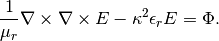
(1)
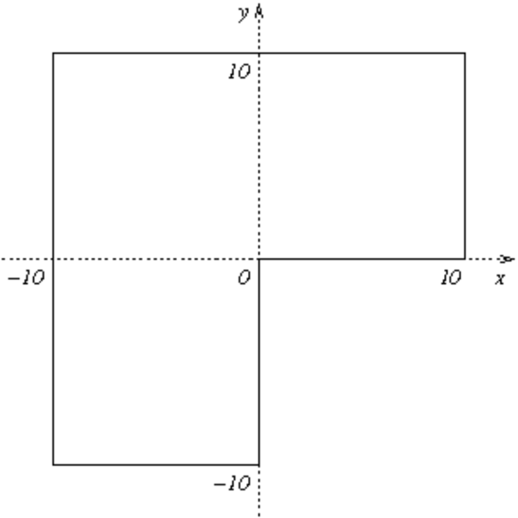
Domain of interest is the square  missing the quarter lying in the
fourth quadrant. It is filled with air:
missing the quarter lying in the
fourth quadrant. It is filled with air:
Boundary conditions: Combined essential and natural, see the file “main.cpp”.
Exact solution
(2)
where  is the Bessel function of the first kind,
 the polar coordinates and
  .
For the source code of the Bessel function
.
For the source code of the Bessel function  see the file definitions.cpp.
Weak forms
The weak formulation is put together as a combination of default jacobian and residual forms in the Hcurl space, and one custom form that defines the integral of the tangential component of the exact solution along the boundary. For details see files definitions.h and definitions.cpp.
Creating a complex Hcurl space
In this example we use the Hcurl space:
// Create an Hcurl space with default shapeset.
HcurlSpace<std::complex<double> > space(&mesh, &bcs, P_INIT);
Choosing refinement selector for the Hcurl space
We also need to use a refinement selector for the Hcurl space:
// Initialize refinement selector.
HcurlProjBasedSelector selector(CAND_LIST, CONV_EXP, H2DRS_DEFAULT_ORDER);
This is the last explicit occurence of the Hcurl space. The rest of the example is the same as if the adaptivity was done in the H1 space.
Choice of projection norm
The H2D_HCURL_NORM is used automatically for the projection, since the projection takes place in an Hcurl space. The user does not have to worry about this. If needed, the default norm can be overridden in the function OGProjection<double> ogProjection; ogProjection.project_global().
Showing real part of the solution
This is done via a RealFilter:
// View the coarse mesh solution and polynomial orders.
RealFilter real_filter(&sln);
v_view.show(&real_filter);
Calculating element errors for adaptivity
Element errors and the total relative error in percent are calculated using
// Calculate element errors and total error estimate.
info("Calculating error estimate and exact error.");
Adapt<std::complex<double> >* adaptivity = new Adapt<std::complex<double> >(&space);
double err_est_rel = adaptivity->calc_err_est(&sln, &ref_sln) * 100;
Also here, the Hcurl norm is used by default.
Exact error calculation and the ‘solutions_for_adapt’ flag
For the exact error calculation, we say that we do not want the exact error to guide automatic adaptivity:
// Calculate exact error.
bool solutions_for_adapt = false;
double err_exact_rel = adaptivity->calc_err_exact(&sln, &sln_exact,
                                                  solutions_for_adapt) * 100;
Sample results
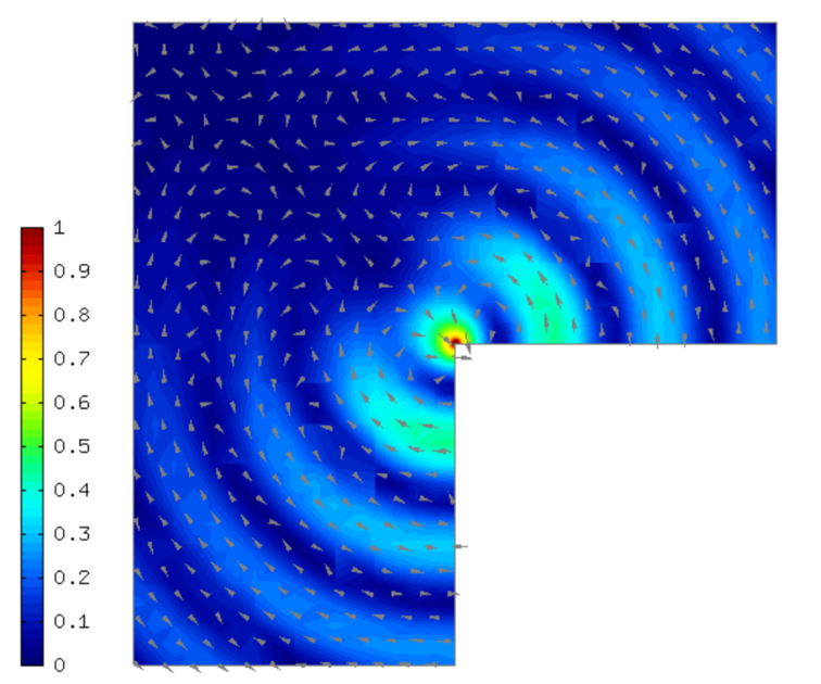
Solution:
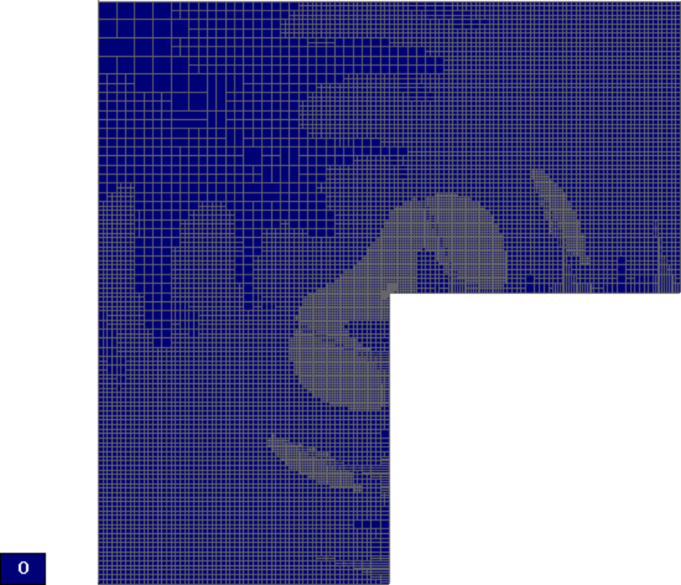
Final mesh (h-FEM with linear elements):
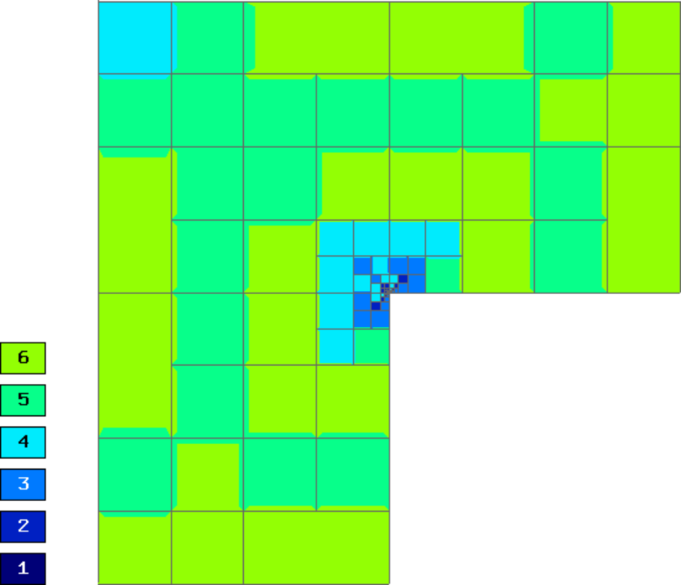
Note that the polynomial order indicated corresponds to the tangential components of approximation on element interfaces, not to polynomial degrees inside the elements (those are one higher).
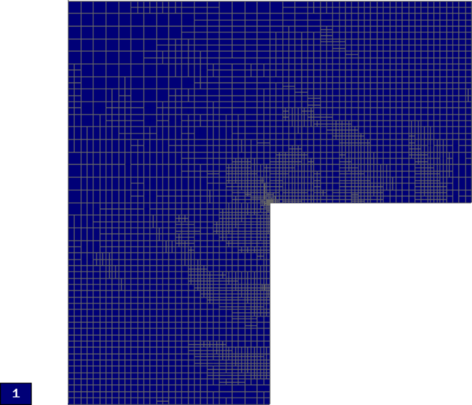
Final mesh (h-FEM with quadratic elements):
Final mesh (hp-FEM):
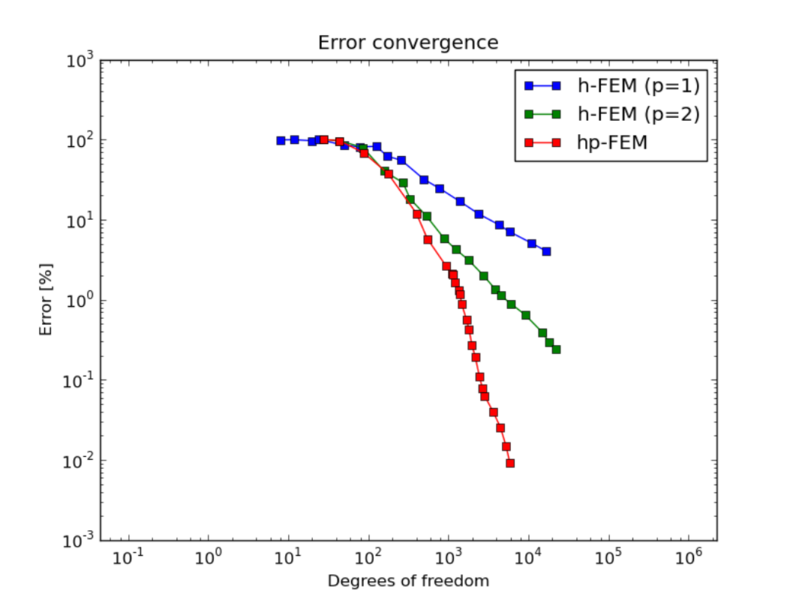
DOF convergence graphs:
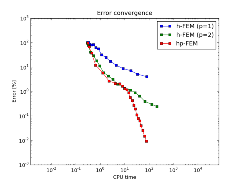
CPU time convergence graphs: