Adaptive Multimesh hp-FEM Example (03-system)
Model problem
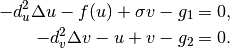
We consider a simplified version of the Fitzhugh-Nagumo equation. This equation is a prominent example of activator-inhibitor systems in two-component reaction-diffusion equations, It describes a prototype of an excitable system (e.g., a neuron) and its stationary form is
Here the unknowns  are the voltage and
  -gate, respectively.
The nonlinear function
-gate, respectively.
The nonlinear function
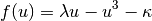
describes how an action potential travels through a nerve. Obviously this system is nonlinear.
Exact solution
In order to make it simpler for this tutorial, we replace the function  with just
  :
:

Our computational domain is the square  and we consider zero Dirichlet conditions
for both and . In order to enable fair convergence comparisons, we will use the following
functions as the exact solution:
and we consider zero Dirichlet conditions
for both and . In order to enable fair convergence comparisons, we will use the following
functions as the exact solution:
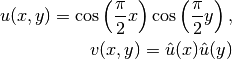
where
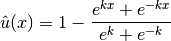
is the exact solution of the one-dimensional singularly perturbed problem
in  , equipped with zero Dirichlet boundary conditions.
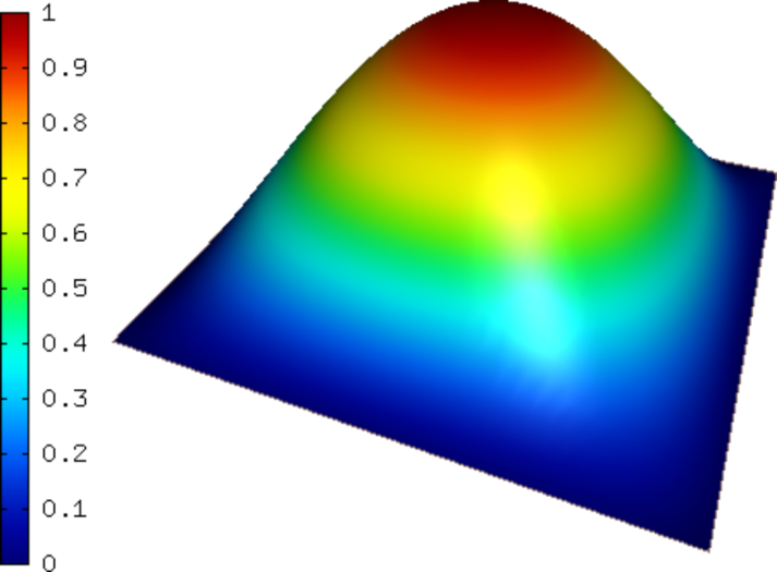
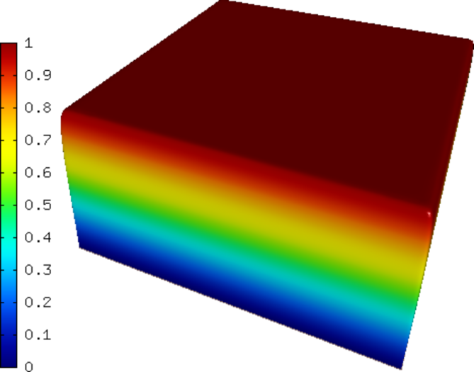
The following two figures show the solutions and . Notice their
large qualitative differences: While is smooth in the entire domain,
has a thin boundary layer along the boundary:
Manufactured right-hand side
The source functions  and
and  are obtained by inserting and
into the PDE system. These functions are not extremely pretty, but they
are not too bad either - see files definitions.h and definitions.cpp.
are obtained by inserting and
into the PDE system. These functions are not extremely pretty, but they
are not too bad either - see files definitions.h and definitions.cpp.
Weak forms
The weak forms can be found in the files definitions.h and definitions.cpp. Beware that although each of the forms is actually symmetric, one cannot use the HERMES_SYM flag as in the elasticity equations, since it has a different meaning.
Adaptivity loop
The adaptivity workflow is standard. First we construct the reference spaces:
// Construct globally refined reference mesh and setup reference space.
Hermes::vector<Space<double> *>* ref_spaces =
  Space<double>::construct_refined_spaces(Hermes::vector<Space<double> *>(&u_space, &v_space));
Next we pass the new reference Spaces to the Newton solver:
newton.set_spaces(ref_spaces);
And we solve the problem using the Newton’s method:
// Perform Newton's iteration.
try
{
  newton.solve(coeff_vec);
}
catch(Hermes::Exceptions::Exception e)
{
  e.printMsg();

}
Next we translate the coefficient vector into the two Solutions, project reference solutions to the coarse meshes, calculate error estimates, calculate exact errors (optional), and adapt the coarse meshes. For details on the last steps see the filemain.cpp.
Sample results
Now we can show some numerical results.
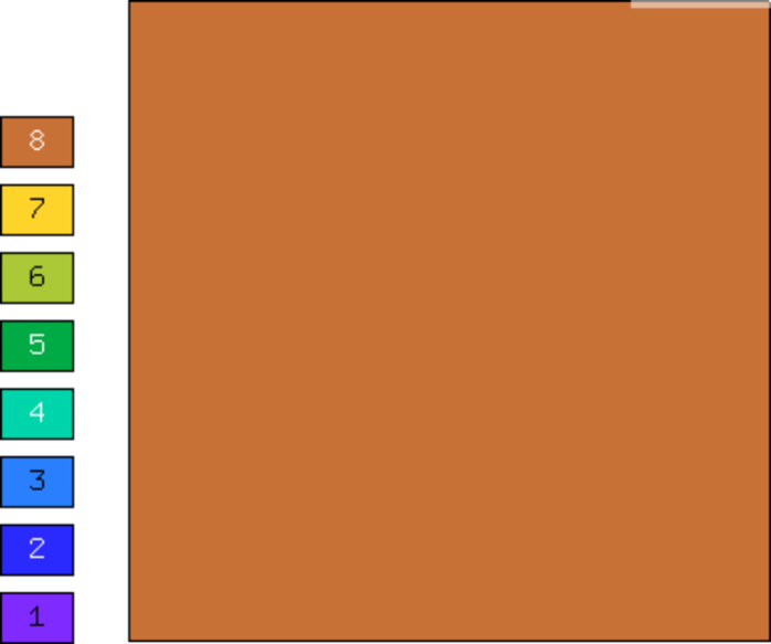
First let us show the resulting meshes for and obtained using
conventional (single-mesh) hp-FEM: 9,330 DOF (4665 for each solution component).
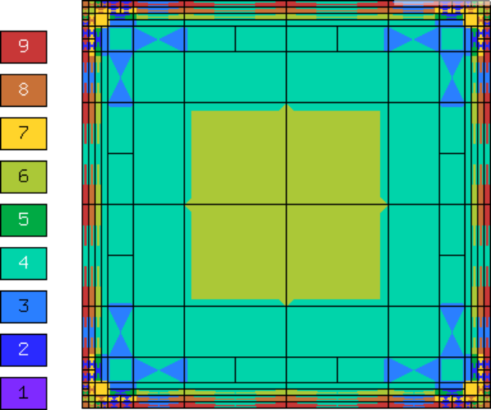
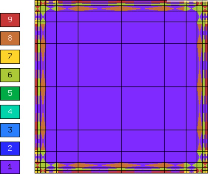
Next we show the resulting meshes for and obtained using
the multimesh hp-FEM: 1,723 DOF (49 DOF for and  for ).
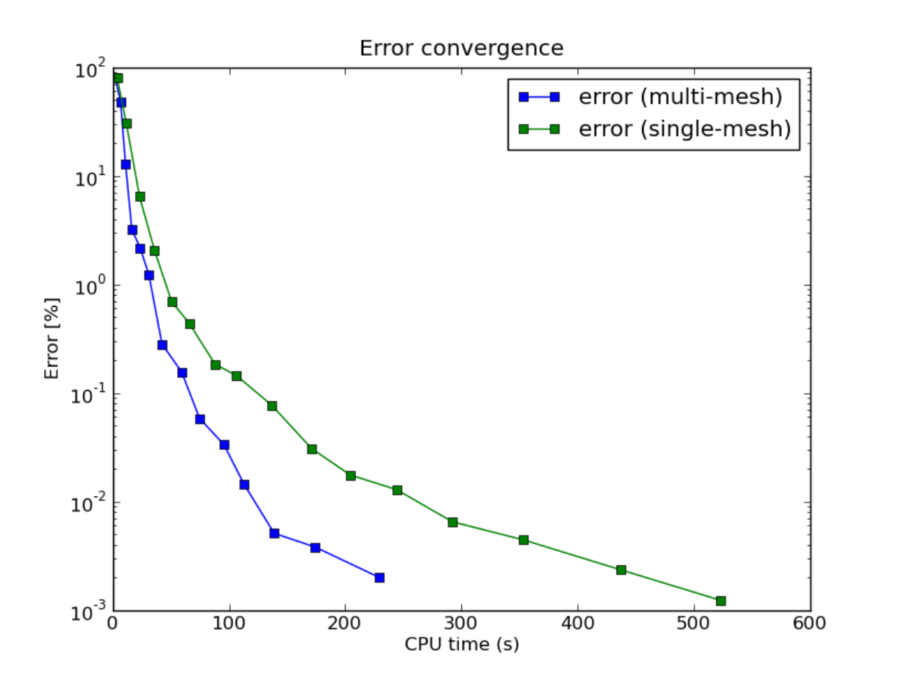
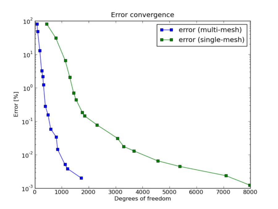
Finally let us compare the DOF and CPU convergence graphs for both cases:
DOF convergence graphs:
CPU time convergence graphs: