Picard’s Method with Acceleration (01-picard)
Picard’s method
The Picard’s method is a simple approach to the solution of nonlinear problems
where nonlinear products are linearized by moving part of the nonlinearity
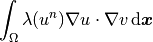
to the previous iteration level. For example, a nonlinear product of the form
 would be linearized as
Anderson acceleration
The Anderson acceleration technique (Anderson mixing) is an old method used in quantum chemistry and other fields, whose aim is to improve the convergence of the Picard’s method by using more than one previous solution. The previous solutions are combined to minimize the least-squares norm under an additional condition saying that the coefficients of the linear combination sum up to 1.0. Besides the implementation in Hermes, you can learn this technique using the Published Worksheet Fixed Point Iteration Method with Acceleration in NCLab.
Model problem
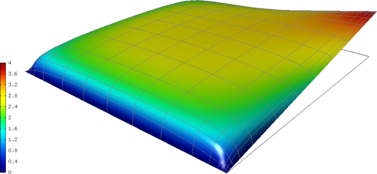
We solve a nonlinear equation

where

One possible interpretation of this equation is stationary heat transfer where the thermal
conductivity  depends on the temperature
  , and
, and  are heat sources/losses.
Our domain is a square
are heat sources/losses.
Our domain is a square 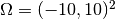 ,
,  , and the nonlinearity has the form
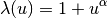
where  is an even nonnegative integer. We will use
  .
Recall that must be entirely positive or entirely negative for the problem to be solvable
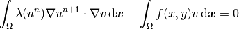
according to the theory. The linearized equation has the form
.
Recall that must be entirely positive or entirely negative for the problem to be solvable
according to the theory. The linearized equation has the form

The Picard’s iteration begins from some initial guess  , in our case a constant
function, and runs until a convergence criterion is satisfied. Most widely used
convergence criteria are the relative error between two consecutive iterations, or
residual of the equation. In this example we will use the former.
, in our case a constant
function, and runs until a convergence criterion is satisfied. Most widely used
convergence criteria are the relative error between two consecutive iterations, or
residual of the equation. In this example we will use the former.
Recall that Hermes uses the Newton’s method to solve linear problems. Therefore, the linearized equation is written as

The residual weak form reads
where  is a given function,
  the approximate solution, and
  a test function. The weak form of the Jacobian is then
where is a given function, a basis function, and a test function.
Defining custom nonlinearity
The nonlinearity is defined by subclassing the Hermes1DFunction class:
class CustomNonlinearity : public Hermes1DFunction<double>
{
public:
  CustomNonlinearity(double alpha);

  virtual double value(double u) const;

  virtual Ord value(Ord u) const;

  protected:
    double alpha;
};
For more details see definitions.cpp.
Defining initial condition
This example uses a constant initial guess:
// Initialize previous iteration solution for the Picard's method.
CustomInitialCondition sln_prev_iter(&mesh, INIT_COND_CONST);
Defining custom weak forms
The weak forms are custom because of containing the previous iteration level solution (see definitions.h and definitions.cpp). Note that the previous iteration level solution is accessed through ext->fn[0];
Initializing the weak formulation
The weak formulation is then initialized in the main.cpp file:
// Initialize the weak formulation.
CustomNonlinearity lambda(alpha);
Hermes2DFunction<double> src(-heat_src);
CustomWeakFormPicard wf(&sln_prev_iter, &lambda, &src);
Picard’s iteration loop
Next we initialize the Picard solver in one of possible ways::and perform the iteration loop:
// 1 - Initialize the Picard solver with a DiscreteProblemLinear.
            DiscreteProblemLinear<double> dp(&wf, &space);
PicardSolver<double> picard(&dp, &sln_prev_iter);

            // 2 - Initialize the Picard solver with WeakForm<double> and Space(s) directly.
PicardSolver<double> picard(&wf, &space, &sln_prev_iter);

            // Some parameter adjustments (if necessary)
            picard.set_picard_tol(PICARD_TOL);
            picard.set_picard_max_iter(PICARD_MAX_ITER);
            picard.set_num_last_iter(PICARD_NUM_LAST_ITER_USED);
            picard.set_anderson_beta(PICARD_ANDERSON_BETA);
To perform an iteration one uses:
// Perform the Picard's iteration (Anderson acceleration on by default).
try
            {
                    picard.solve();
            }
            catch(std::exception& e)
            {
                    std::cout << e.what();
            }
Here PICARD_NUM_LAST_ITER_USED is the number of last iterates to use for the acceleration. With PICARD_NUM_LAST_ITER_USED = 1 one has the original Picard’s method. The parameter PICARD_ANDERSON_BETA also influences the convergence of the accelerated method but there is no recipe how to choose it - you can either experiment with it or set it to zero.
Convergence of the original method
The convergence of the original Picard’s method with PICARD_NUM_LAST_ITER_USED = 1 is not fast:
I ---- Picard iter 1, ndof 1225, rel. error 0.141587%
I ---- Picard iter 2, ndof 1225, rel. error 0.137839%
I ---- Picard iter 3, ndof 1225, rel. error 0.108533%
I ---- Picard iter 4, ndof 1225, rel. error 0.0924885%
I ---- Picard iter 5, ndof 1225, rel. error 0.082466%
I ---- Picard iter 6, ndof 1225, rel. error 0.0630463%
I ---- Picard iter 7, ndof 1225, rel. error 0.0728757%
I ---- Picard iter 8, ndof 1225, rel. error 0.054595%
I ---- Picard iter 9, ndof 1225, rel. error 0.051211%
I ---- Picard iter 10, ndof 1225, rel. error 0.053429%
I ---- Picard iter 11, ndof 1225, rel. error 0.0380756%
I ---- Picard iter 12, ndof 1225, rel. error 0.0417355%
I ---- Picard iter 13, ndof 1225, rel. error 0.033854%
I ---- Picard iter 14, ndof 1225, rel. error 0.0310395%
I ---- Picard iter 15, ndof 1225, rel. error 0.0308319%
I ---- Picard iter 16, ndof 1225, rel. error 0.0230805%
I ---- Picard iter 17, ndof 1225, rel. error 0.0268781%
I ---- Picard iter 18, ndof 1225, rel. error 0.0211553%
I ---- Picard iter 19, ndof 1225, rel. error 0.0196746%
I ---- Picard iter 20, ndof 1225, rel. error 0.0205413%
I ---- Picard iter 21, ndof 1225, rel. error 0.0149323%
I ---- Picard iter 22, ndof 1225, rel. error 0.0167516%
I ---- Picard iter 23, ndof 1225, rel. error 0.0136722%
I ---- Picard iter 24, ndof 1225, rel. error 0.012374%
I ---- Picard iter 25, ndof 1225, rel. error 0.0127109%
I ---- Picard iter 26, ndof 1225, rel. error 0.00938446%
I ---- Picard iter 27, ndof 1225, rel. error 0.0107242%
I ---- Picard iter 28, ndof 1225, rel. error 0.00869685%
I ---- Picard iter 29, ndof 1225, rel. error 0.00785618%
I ---- Picard iter 30, ndof 1225, rel. error 0.00828885%
I ---- Picard iter 31, ndof 1225, rel. error 0.00603982%
I ---- Picard iter 32, ndof 1225, rel. error 0.00678621%
I ---- Picard iter 33, ndof 1225, rel. error 0.00562285%
I ---- Picard iter 34, ndof 1225, rel. error 0.00497509%
I ---- Picard iter 35, ndof 1225, rel. error 0.00524203%
I ---- Picard iter 36, ndof 1225, rel. error 0.00384045%
I ---- Picard iter 37, ndof 1225, rel. error 0.00432833%
I ---- Picard iter 38, ndof 1225, rel. error 0.00359952%
I ---- Picard iter 39, ndof 1225, rel. error 0.00315926%
I ---- Picard iter 40, ndof 1225, rel. error 0.00338247%
I ---- Picard iter 41, ndof 1225, rel. error 0.00246534%
I ---- Picard iter 42, ndof 1225, rel. error 0.00274954%
I ---- Picard iter 43, ndof 1225, rel. error 0.00232243%
I ---- Picard iter 44, ndof 1225, rel. error 0.00200454%
I ---- Picard iter 45, ndof 1225, rel. error 0.00215508%
I ---- Picard iter 46, ndof 1225, rel. error 0.00157491%
I ---- Picard iter 47, ndof 1225, rel. error 0.00175017%
I ---- Picard iter 48, ndof 1225, rel. error 0.00149047%
I ---- Picard iter 49, ndof 1225, rel. error 0.00127281%
I ---- Picard iter 50, ndof 1225, rel. error 0.00138365%
I ---- Picard iter 51, ndof 1225, rel. error 0.00101007%
I ---- Picard iter 52, ndof 1225, rel. error 0.00111257%
I ---- Picard iter 53, ndof 1225, rel. error 0.000960116%
Convergence of the original method
The convergence of the accelerated method with PICARD_NUM_LAST_ITER_USED = 4 and PICARD_ANDERSON_BETA = 0.2 looks as follows:
I ---- Picard iter 1, ndof 1225, rel. error 0.141587%
I ---- Picard iter 2, ndof 1225, rel. error 0.137839%
I ---- Picard iter 3, ndof 1225, rel. error 0.0811892%
I ---- Picard iter 4, ndof 1225, rel. error 0.0332969%
I ---- Picard iter 5, ndof 1225, rel. error 0.0258267%
I ---- Picard iter 6, ndof 1225, rel. error 0.00796399%
I ---- Picard iter 7, ndof 1225, rel. error 0.0110749%
I ---- Picard iter 8, ndof 1225, rel. error 0.000181404%