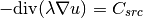
Poisson Equation (03-poisson)
This example shows how to solve a simple PDE that describes stationary heat transfer in an object that is heated by constant volumetric heat sources (such as with a DC current). The temperature equals to a prescribed constant on the boundary. We will learn how to:
- Define a weak formulation.
- Select a matrix solver.
- Solve the discrete problem.
- Output the solution and element orders in VTK format (to be visualized, e.g., using Paraview).
- Visualize the solution using Hermes native OpenGL functionality.
Model problem
Consider the Poisson equation
(1)
in the L-shaped domain  from the previous examples.
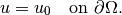
The equation is equipped with constant Dirichlet boundary conditions
from the previous examples.
The equation is equipped with constant Dirichlet boundary conditions
(2)
Here  is an unknown temperature distribution,
 a real number representing volumetric heat sources/losses, and
  is thermal conductivity
of the material.
is thermal conductivity
of the material.
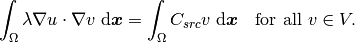
The weak formulation is derived as usual, first by multiplying equation (1)
with a test function  , then integrating over the domain , and then applying
the Green’s theorem (integration by parts) to the second derivatives.
Because of the Dirichlet condition (2),
there are no surface integrals. Since the product of the two gradients
in the volumetric weak form needs to be integrable for all and in
, then integrating over the domain , and then applying
the Green’s theorem (integration by parts) to the second derivatives.
Because of the Dirichlet condition (2),
there are no surface integrals. Since the product of the two gradients
in the volumetric weak form needs to be integrable for all and in  ,
the proper space for the solution is
,
the proper space for the solution is  . The weak formulation
reads: Find
. The weak formulation
reads: Find  such that
(3)
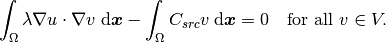
Hermes, however, expects the equation in the form
(4)
Let us explain why.
Jacobian-residual formulation
Hermes always assumes that the problem is nonlinear, and by default it uses the Newton’s method to solve it. Other methods for the solution of nonlinear problems are available as well (to be discussed later).
For linear problems, the Newton’s method converges in one step - the theory says.
In practice the Newton’s method may take more than one step for a linear problem if the matrix solver does not do a good job. This is not unusual at all, in particular when an iterative solver is used. By checking the residual of the equation, the Newton’s method always makes sure that the problem is solved correctly, or it fails in a transparent way. This is the main reason why Hermes employs the Newton’s method even for problems that are linear.
Another reason is that a consistent approach to linear and nonlinear problems allows the users to first formulate and solve a simplified linear version of the problem, and then upgrade it to a full nonlinear version effortlessly. Let’s explain how this works.
Consistent approach to linear and nonlinear problems
This is an approach to linear problems as to nonlinear ones (I.e. using Newton’s method for linear problems as well). That would be the section ‘1 - nonlinear formulation’ further down on this page. However, in the section ‘2 - linear formulation’, the linear approach one can also use is explained.
First assume that  in
in  and
and
 in
in  where both
  and
and  are constants. Then the problem is linear and the weak form for the Jacobian is
where stands for a basis function and for a test function.
The reader does not have to worry about the word “Jacobian” here since for linear
problems it is the same as “stiffness matrix”. Simply forget from the left-hand side
of the weak formulation (4) all expressions that do not contain .
A detailed explanation of the Newton’s method for nonlinear problems will be provided
at the beginning of the tutorial part P02.
The residual weak form is the entire left-hand side of (4) where
is now the approximate solution (not a basis function as above):

This is the constructor of the corresponding weak formulation in Hermes:
CustomWeakFormPoisson::CustomWeakFormPoisson(std::string mat_al, Hermes1DFunction<double>* lambda_al,
                                         std::string mat_cu, Hermes1DFunction<double>* lambda_cu,
                                         Hermes2DFunction<double>* src_term) : WeakForm<double>(1)
{
  // Jacobian forms.
  add_matrix_form(new DefaultJacobianDiffusion<double>(0, 0, mat_al, lambda_al));
  add_matrix_form(new DefaultJacobianDiffusion<double>(0, 0, mat_cu, lambda_cu));

  // Residual forms.
  add_vector_form(new DefaultResidualDiffusion<double>(0, mat_al, lambda_al));
  add_vector_form(new DefaultResidualDiffusion<double>(0, mat_cu, lambda_cu));
  add_vector_form(new DefaultVectorFormVol<double>(0, HERMES_ANY, src_term));
};
Here HERMES_ANY means that the volumetric vector form will be assigned to all material markers.
For constant lambda_al and lambda_cu, the form is instantiated as follows:
CustomWeakFormPoisson wf("Aluminum", new Hermes1DFunction<double>(lambda_al), "Copper",
                         new Hermes1DFunction<double>(lambda_cu),
                         new Hermes2DFunction<double>(-src_term));
Once a linear version of a problem works, it is very easy to extend it to a nonlinear case. For example, to replace the constants with cubic splines, one just needs to do
CubicSpline lambda_al(...);
CubicSpline lambda_cu(...);
CustomWeakFormPoisson wf("Aluminum", &lambda_al, "Copper",
                         &lambda_cu, new Hermes2DFunction<double>(-src_term));
This is possible since CubicSpline is a descendant of Hermes1DFunction. Analogously, the
constant src_term can be replaced with an arbitrary function of  and
and  by
subclassing Hermes2DFunction:
by
subclassing Hermes2DFunction:
class CustomNonConstSrc<Scalar> : public Hermes2DFunction<Scalar>
...
If cubic splines are not enough, then one can subclass Hermes1DFunction to define arbitrary nonlinearities:
class CustomLambdaAl<Scalar> : public Hermes1DFunction<Scalar>
...
class CustomLambdaCu<Scalar> : public Hermes1DFunction<Scalar>
...
In the rest of part P01 we will focus on linear problems.
Default Jacobian for the diffusion operator
Hermes provides default weak forms for many common PDE operators. To begin with, the line
add_matrix_form(new DefaultJacobianDiffusion<double>(0, 0, marker_al, lambda_al));
adds to the Jacobian weak form the integral
where is a basis function and a test function.
It has the following constructors:
DefaultJacobianDiffusion(int i = 0, int j = 0, std::string area = HERMES_ANY,
                         Hermes1DFunction<Scalar>* coeff = HERMES_ONE,
                         SymFlag sym = HERMES_NONSYM, GeomType gt = HERMES_PLANAR);
and
DefaultJacobianDiffusion(int i = 0, int j = 0, Hermes::vector<std::string> areas,
                         Hermes1DFunction<Scalar>* coeff = HERMES_ONE,
                         SymFlag sym = HERMES_NONSYM, GeomType gt = HERMES_PLANAR);
The pair of indices ‘i’ and ‘j’ identifies a block in the Jacobian matrix (for systems of equations). For a single equation it is i = j = 0.
The parameter ‘area’ identifies the material marker of elements to which the weak form will be assigned. HERMES_ANY means to any material marker.
The parameter ‘coeff’ can be a constant, cubic spline, or a general nonlinear function
of the solution . HERMES_ONE means constant 1.0.
SymFlag is the symmetry flag. If SymFlag sym == HERMES_NONSYM, then Hermes evaluates the form at both symmetric positions r, s and s, r in the stiffness matrix. If sym == HERMES_SYM, only the integral at the position r, s is evaluated, and its value is copied to the symmetric position s, r. If sym == HERMES_ANTISYM, the value is copied with a minus sign.
The GeomType parameter tells Hermes whether the form is planar (HERMES_PLANAR), axisymmetrix with respect to the x-axis (HERMES_AXISYM_X), or axisymmetrix with respect to the y-axis (HERMES_AXISYM_Y).
The form can be linked to multiple material markers:
DefaultJacobianDiffusion(int i, int j, Hermes::vector<std::string> areas,
                         Hermes1DFunction<Scalar>* coeff = HERMES_ONE,
                         SymFlag sym = HERMES_NONSYM, GeomType gt = HERMES_PLANAR);
Here, Hermes::vector is just a std::vector equipped with additional constructors for comfort. Sample usage:
Hermes::vector<std::string> areas("marker_1", "marker_2", "marker_3");
Default residual for the diffusion operator
Similarly, the line
add_vector_form(new DefaultResidualDiffusion<double>(0, marker_al, lambda_al));
adds to the residual weak form the integral
where is the approximate solution and a test function.
Default volumetric vector form
The last default weak form used in the CustomWeakFormPoisson class above is
add_vector_form(new DefaultVectorFormVol<double>(0, HERMES_ANY, c));
It adds to the residual weak form the integral

and thus it completes (4).
Selecting matrix solver
Before the main function, one needs to choose a matrix solver:
Hermes::HermesCommonApi.setParamValue(Hermes::matrixSolverType, Hermes::SOLVER_UMFPACK);
Besides UMFPACK, one can use SOLVER_AMESOS, SOLVER_MUMPS, SOLVER_PETSC, and SOLVER_SUPERLU. Matrix-free SOLVER_NOX for nonlinear problems will be discussed later.
Loading the mesh
The main.cpp file begins with loading the mesh. In many examples including this one, the mesh is available both in the native Hermes format and the Hermes XML format:
// Load the mesh.
Mesh mesh;
if (USE_XML_FORMAT == true)
{
  MeshReaderH2DXML mloader;
  info("Reading mesh in XML format.");
  mloader.load("domain.xml", &mesh);
}
else
{
  MeshReaderH2D mloader;
  info("Reading mesh in original format.");
  mloader.load("domain.mesh", &mesh);
}
Performing initial mesh refinements
A number of initial refinement operations can be done as explained in example P01/01-mesh. In this case we just perform optional uniform mesh refinements:
// Perform initial mesh refinements (optional).
for (int i = 0; i < INIT_REF_NUM; i++)
  mesh.refine_all_elements();
Initializing the weak formulation
Next, an instance of the corresponding weak form class is created:
// Initialize the weak formulation.
CustomWeakFormPoisson wf("Aluminum", new Hermes1DFunction<double>(lambda_al), "Copper",
                         new Hermes1DFunction<double>(lambda_cu), new Hermes2DFunction<double>(-src_term));
Setting constant Dirichlet boundary conditions
Constant Dirichlet boundary conditions are assigned to the boundary markers “Bottom”, “Inner”, “Outer”, and “Left” as follows:
// Initialize essential boundary conditions.
DefaultEssentialBCConst<double> bc_essential(Hermes::vector<std::string>("Bottom", "Inner", "Outer", "Left"),
                                             FIXED_BDY_TEMP);
EssentialBCs<double> bcs(&bc_essential);
Do not worry about the complicated-looking Hermes::vector, this is just std::vector enhanced with a few extra constructors. It is used to avoid using variable-length arrays.
The treatment of nonzero Dirichlet and other boundary conditions will be explained in more detail in the following examples. For the moment, let’s proceed to the finite element space.
Initializing finite element space
As a next step, we initialize the FE space in the same way as in the previous tutorial example 02-space:
// Create an H1 space with default shapeset.
H1Space<double> space(&mesh, &bcs, P_INIT);
Here P_INIT is a uniform polynomial degree of mesh elements (an integer number between 1 and 10).
1 - nonlinear formulation
In the following, the problem is solved with the use of the Newton’s method, althought it is linear, to demonstrate the differences. The linear formulation follows after.
Initializing discrete problem
The weak formulation and finite element space(s) constitute a finite element problem. To define it, one needs to create an instance of the DiscreteProblem class:
// Initialize the FE problem.
DiscreteProblem<double> dp(&wf, &space);
Initializing Newton solver
The Newton solver class is initialized using a pointer to DiscreteProblem and the matrix solver:
// Initialize Newton solver.
NewtonSolver<double> newton(&dp);
One can also directly use the following constructor, without creating an instance of DiscreteProblem first:
// Initialize Newton solver.
NewtonSolver<double> newton(&wf, &space);
Performing the Newton’s iteration
Next, the Newton’s method is employed in an exception-safe way. For a linear problem, it usually only takes one step, but sometimes it may take more if the matrix is ill-conditioned or if for any other reason the residual after the first step is not under the prescribed tolerance. If all arguments are skipped in newton.solve(), this means that the Newton’s method will start from a zero initial vector, with a default tolerance 1e-8, and with a default maximum allowed number of 100 iterations:
// Perform Newton's iteration.
try
{
  newton.solve();
}
catch(Hermes::Exceptions::Exception e)
{
  e.printMsg();

}
The method solve() comes in two basic versions:
void solve(Scalar* coeff_vec = NULL);
void solve_keep_jacobian(Scalar* coeff_vec = NULL);
The latter keeps the Jacobian constant during the Newton’s iteration loop. Their detailed description, as well as additional useful methods of the NewtonSolver class, are described in the Doxygen documentation.
Translating the coefficient vector into a solution
The coefficient vector can be converted into a piecewise-polynomial Solution via the function Solution<Scalar>::vector_to_solution():
// Translate the resulting coefficient vector into a Solution.
Solution<double> sln;
Solution<double>::vector_to_solution(newton.get_sln_vector(), &space, &sln);
2 - linear formulation
Here the problem is solved as a linear one. We do not need to adjust the weak formulation we used for the Newton’s method, as in the linear setting, the previous Newton’s iterations will be set to zero.
Initializing linear solver
Again, the weak formulation and finite element space(s) constitute a finite element problem. We can use one of the following ways to create a LinearSolver:
// Initialize the FE problem.
DiscreteProblem<double> dp(&wf, &space);
// Use it in the constructor of the solver.
LinearSolver<double> linear_solver(&dp);

// Use directly the weak formulation and the space(s).
LinearSolver<double> linear_solver(&wf, &space);
Solving
In the same way as in the Newton’s method, there is a method solve():
void LinearSolver::solve();
We can see that the linear solver is more lightweight to use than the Newton’s method.
Translating the coefficient vector into a solution
As before, the coefficient vector can be converted into a piecewise-polynomial Solution via the function Solution<Scalar>::vector_to_solution():
// Translate the resulting coefficient vector into a Solution.
Solution<double> sln;
Solution<double>::vector_to_solution(linear_solver.get_sln_vector(), &space, &sln);
Visualization
Saving solution in VTK format
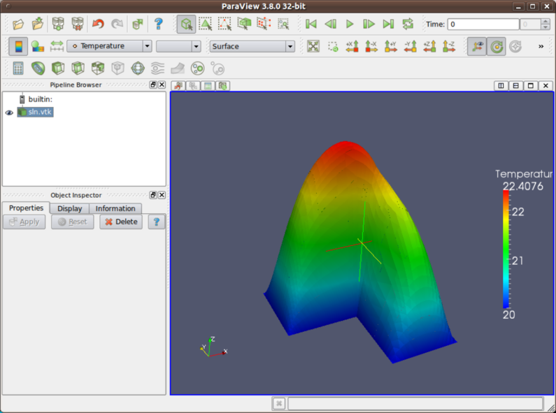
The solution can be saved in the VTK format to be visualized, for example, using Paraview. To do this, one uses the Linearizer class that has the ability to approximate adaptively a higher-order polynomial solution using linear triangles:
// VTK output.
if (VTK_VISUALIZATION)
{
  // Output solution in VTK format.
  Linearizer lin;
  bool mode_3D = true;
  lin.save_solution_vtk(&sln, "sln.vtk", "Temperature", mode_3D);
  info("Solution in VTK format saved to file %s.", "sln.vtk");

  // Output mesh and element orders in VTK format.
  Orderizer ord;
  ord.save_orders_vtk(&space, "ord.vtk");
  info("Element orders in VTK format saved to file %s.", "ord.vtk");
}
The full header of the method save_solution_vtk() can be found in Doxygen documentation. Only the first three arguments are mandatory and there is a number of optional parameters whose meaning is as follows:
- mode_3D ... select either 2D or 3D rendering (default is 3D).
- item: H2D_FN_VAL_0 ... show function values, H2D_FN_DX_0 ... show x-derivative, H2D_FN_DY_0 ... show y-derivative, H2D_FN_DXX_0 ... show xx-derivative, H2D_FN_DXY_0 ... show xy-derivative, H2D_FN_DYY_0 ... show yy-derivative,
- eps: HERMES_EPS_LOW ... low resolution (small output file), HERMES_EPS_NORMAL ... normal resolution (medium output file), HERMES_EPS_HIGH ... high resolution (large output file), HERMES_EPS_VERYHIGH ... high resolution (very large output file).
- max_abs: technical parameter, see file src/linearizer/linear.h.
- xdisp, ydisp, dmult: Can be used to deform the domain. Typical applications are elasticity, plasticity, etc.
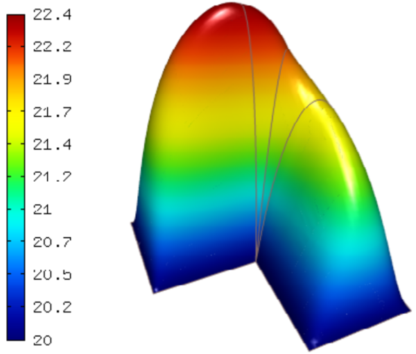
The following figure shows the corresponding Paraview visualization:
Visualizing the solution using OpenGL
The solution can also be visualized via the ScalarView class:
// Visualize the solution.
ScalarView view("Solution", new WinGeom(0, 0, 440, 350));
view.show(&sln, HERMES_EPS_HIGH);
View::wait();
Hermes’ built-in OpenGL visualization looks as follows:
Visualization quality
The method show() has an optional second parameter – the visualization accuracy. It can have the values HERMES_EPS_LOW, HERMES_EPS_NORMAL (default), HERMES_EPS_HIGH and HERMES_EPS_VERYHIGH. This parameter influences the number of linear triangles that Hermes uses to approximate higher-order polynomial solutions with linear triangles for OpenGL. In fact, the EPS value is a stopping criterion for automatic adaptivity that Hermes uses to keep the number of the linear triangles as low as possible.
If you notice in the image white points or even discontinuities
where the approximation is continuous, try to move from HERMES_EPS_NORMAL to
HERMES_EPS_HIGH. If the interval of solution values is very small compared to
the solution magnitude, such as if the solution values lie in the interval
 , then you may need HERMES_EPS_VERYHIGH.
Before pressing ‘s’ to save the image, make sure to press ‘h’ to render high-quality image.
Visualization of derivatives
The method show() also has an optional third parameter to indicate whether function values or partial derivatives should be displayed. For example, HERMES_FN_VAL_0 stands for the function value of solution component 0 (first solution component which in this case is the VonMises stress). HERMES_FN_VAL_1 would mean the function value of the second solution component (relevant for vector-valued Hcurl or Hdiv elements only), HERMES_FN_DX_0 means the x-derivative of the first solution component, etc.