Basic-ie-picard
Model problem
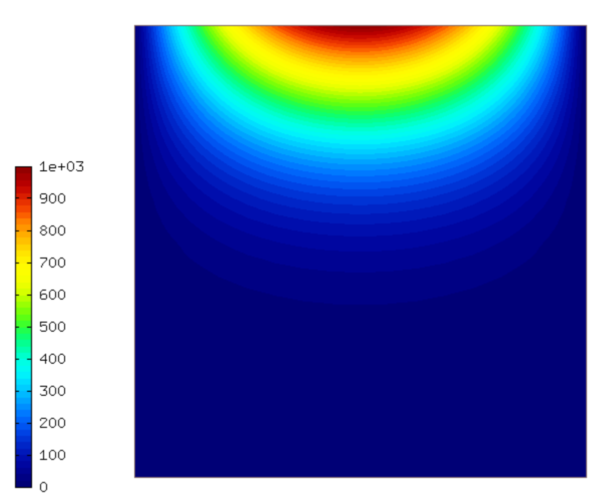
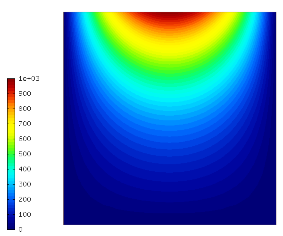
This example is similar to basic-ie-newton except it uses the Picard’s method in each time step (not Newton’s method).
We assume the time-dependent Richard’s equation
(1)
where  and
and  are non-differentiable and thus in some cases the Newton’s method has convergence problems.
For this reason, the Picard’s method is a popular approach. If Picards is used, then Andersson acceleration should be employed.
are non-differentiable and thus in some cases the Newton’s method has convergence problems.
For this reason, the Picard’s method is a popular approach. If Picards is used, then Andersson acceleration should be employed.
equipped with a Dirichlet, given by the initial condition.

The pressure head ‘h’ is between -1000 and 0. For convenience, we increase it by an offset H_OFFSET = 1000. In this way we can start from a zero coefficient vector.
Weak formulation
The corresponding weak formulation reads

Here  refers to time steps and
  to Picard’s iterations within one time step.
Defining weak forms
The weak formulation is a combination of custom Jacobian and Residual weak forms:
CustomWeakFormRichardsIEPicard::CustomWeakFormRichardsIEPicard(double time_step, Solution* h_time_prev, Solution* h_iter_prev) : WeakForm<double>(1)
{
  // Jacobian.
  CustomJacobian* matrix_form = new CustomJacobian(0, 0, time_step);
  matrix_form->ext.push_back(h_time_prev);
  matrix_form->ext.push_back(h_iter_prev);
  add_matrix_form(matrix_form);

  // Residual.
  CustomResidual* vector_form = new CustomResidual(0, time_step);
  vector_form->ext.push_back(h_time_prev);
  vector_form->ext.push_back(h_iter_prev);
  add_vector_form(vector_form);
}