Circular-Obstacle
Model problem
In this example, the time-dependent laminar incompressible Navier-Stokes equations are
discretized in time via the implicit Euler method. If NEWTON == true,
the Newton’s method is used to solve the nonlinear problem at each time
step. If NEWTON == false, the convective term only is linearized using the
velocities from the previous time step. Obviously the latter approach is wrong,
but people do this frequently because it is faster and simpler to implement.
Therefore we include this case for comparison purposes. We also show how
to use discontinuous ( ) elements for pressure and thus make the
velocity discreetely divergence free. Comparison to approximating the
pressure with the standard (continuous) Taylor-Hood elements is shown.
) elements for pressure and thus make the
velocity discreetely divergence free. Comparison to approximating the
pressure with the standard (continuous) Taylor-Hood elements is shown.
The computational domain is a rectangular channel containing a circular obstacle:
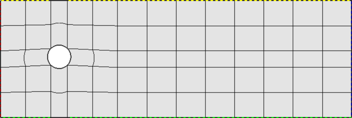
The circle is defined via NURBS. Its radius and position, as well as some additional geometry parameters can be changed in the mesh file “domain.mesh”:
L = 15            # domain length (should be a multiple of 3)
H = 5             # domain height
S1 = 5/2          # x-center of circle
S2 = 5/2          # y-center of circle
R = 1             # circle radius
A = 1/(2*sqrt(2)) # helper length
EPS = 0.10        # vertical shift of the circle
The Navier-Stokes equations are assumed in the standard form
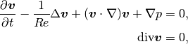
where  is the velocity vector,
  the Reynolds number,
  the pressure,
and
the pressure,
and  the nonlinear convective term. We prescribe a parabolic
velocity profile at inlet (the left-most edge). The inlet velocity is time-dependent, it
increases linearly in time from zero to a user-defined value during an initial time period,
and then it stays constant. Standard no-slip velocity boundary conditions are prescribed
on the rest of the boundary with the exception of the outlet (right-most edge) where the
standard “do nothing” boundary conditions are prescribed. No boundary conditions are
prescribed for pressure - being an -function, the pressure does not
admit any boundary conditions.
the nonlinear convective term. We prescribe a parabolic
velocity profile at inlet (the left-most edge). The inlet velocity is time-dependent, it
increases linearly in time from zero to a user-defined value during an initial time period,
and then it stays constant. Standard no-slip velocity boundary conditions are prescribed
on the rest of the boundary with the exception of the outlet (right-most edge) where the
standard “do nothing” boundary conditions are prescribed. No boundary conditions are
prescribed for pressure - being an -function, the pressure does not
admit any boundary conditions.
Role of pressure in Navier-Stokes equations
The role of the pressure in the Navier-Stokes equations
is interesting and worth a brief discussion. Since the equations only contain its gradient,
it is determined up to a constant. This does not mean that the problem is ill-conditioned
though, since the pressure only plays the role of a Lagrange multiplier that keeps
the velocity divergence-free. More precisely, the better the pressure is resolved,
the closer the approximate velocity to being divergence free. The best one can do
is to approximate the pressure in (using discontinuous elements). Not only because
it is more meaningful from the point of view of the weak formulation, but also because
the approximate velocity automatically becomes discreetely divergence-free (integral
of its divergence over every element in the mesh is zero). The standard Taylor-Hood
elements approximating both the velocity and pressure with  -conforming (continuous)
elements do not have this property and thus are less accurate. We will compare these
two approaches below. Last, the pressure needs to be approximated by elements of
a lower polynomial degree than the velocity in order to satisfy the inf-sup condition.
-conforming (continuous)
elements do not have this property and thus are less accurate. We will compare these
two approaches below. Last, the pressure needs to be approximated by elements of
a lower polynomial degree than the velocity in order to satisfy the inf-sup condition.
The time derivative is approximated using the implicit Euler method:
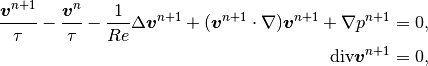
where  is the time step. This is a nonlinear problem that involves three equations (two
for velocity components and the continuity equation).
is the time step. This is a nonlinear problem that involves three equations (two
for velocity components and the continuity equation).
Defining spaces
We define three spaces for the two velocity components and pressure. This is either [H1, H1, H1] or [H1, H1, L2]:
  // Spaces for velocity components and pressure.
  H1Space xvel_space(&mesh, &bcs_vel_x, P_INIT_VEL);
  H1Space yvel_space(&mesh, &bcs_vel_y, P_INIT_VEL);
#ifdef PRESSURE_IN_L2
  L2Space p_space(&mesh, &bcs_pressure, P_INIT_PRESSURE);
#else
  H1Space p_space(&mesh, &bcs_pressure, P_INIT_PRESSURE);
#endif
Defining projection norms
We need to define the proper projection norms in these spaces:
  // Define projection norms.
  ProjNormType vel_proj_norm = HERMES_H1_NORM;
#ifdef PRESSURE_IN_L2
  ProjNormType p_proj_norm = HERMES_L2_NORM;
#else
  ProjNormType p_proj_norm = HERMES_H1_NORM;
#endif
Calculating initial coefficient vector for the Newton’s method
After registering weak forms and initializing the DiscreteProblem, if NEWTON == true
we calculate the initial coefficient vector  for the Newton’s method:
// Project the initial condition on the FE space to obtain initial
// coefficient vector for the Newton's method.
scalar* coeff_vec = new scalar[Space::get_num_dofs(Hermes::vector<Space *>(&xvel_space, &yvel_space, &p_space))];
if (NEWTON) {
  info("Projecting initial condition to obtain initial vector for the Newton's method.");
  OGProjection::project_global(Hermes::vector<Space *>(&xvel_space, &yvel_space, &p_space),
                 Hermes::vector<MeshFunction *>(&xvel_prev_time, &yvel_prev_time, &p_prev_time),
                 coeff_vec, matrix_solver,
                 Hermes::vector<ProjNormType>(vel_proj_norm, vel_proj_norm, p_proj_norm));
}
Note that when projecting multiple functions, we can use different projection norms for each.
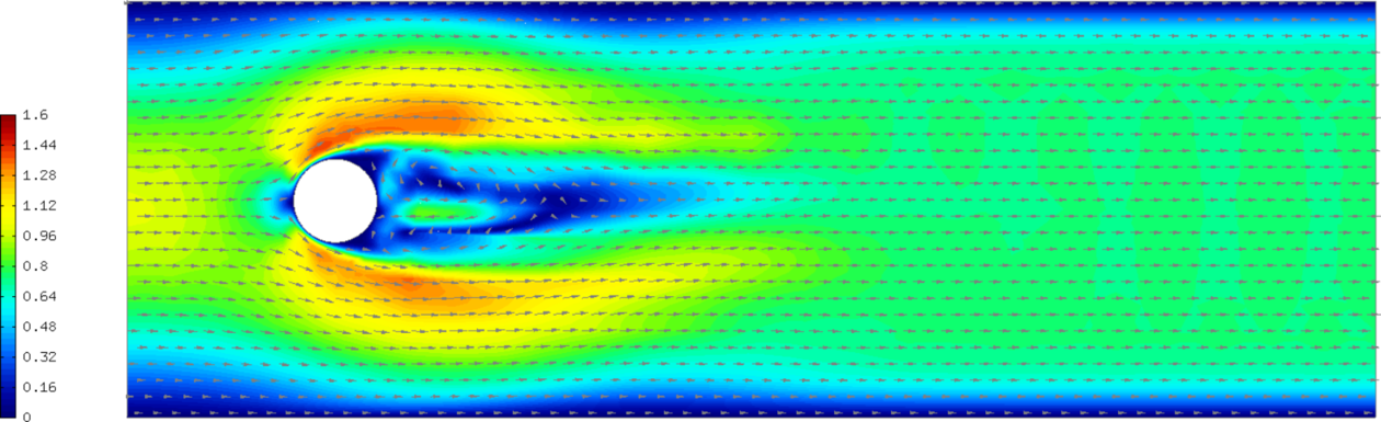
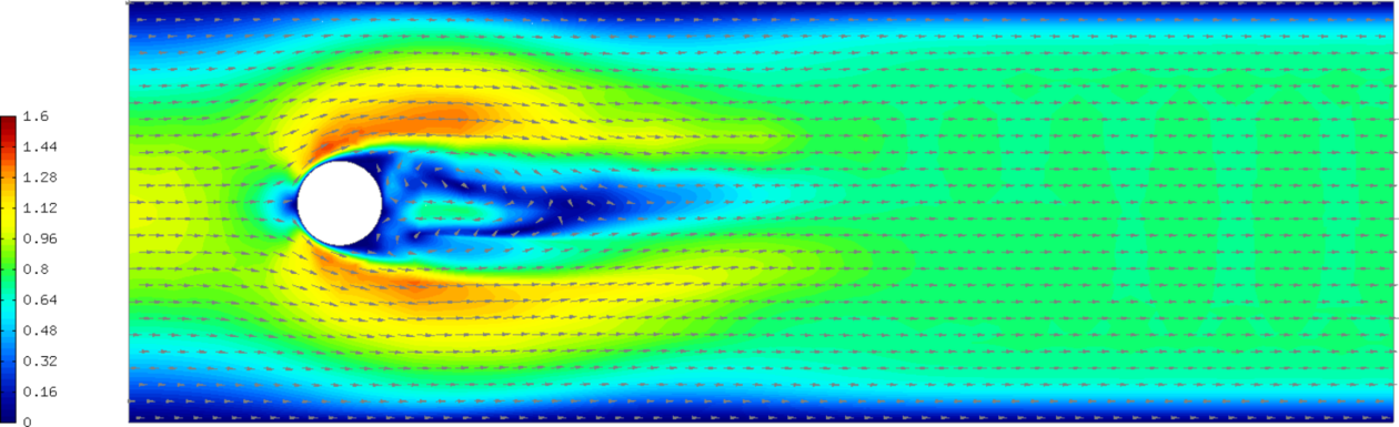
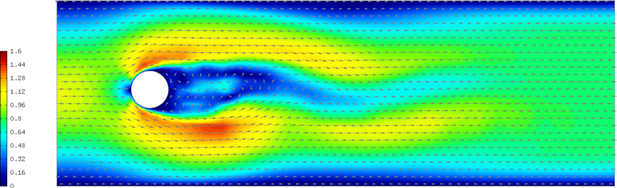
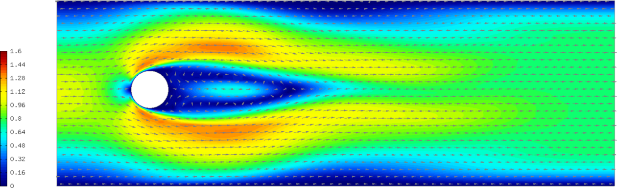
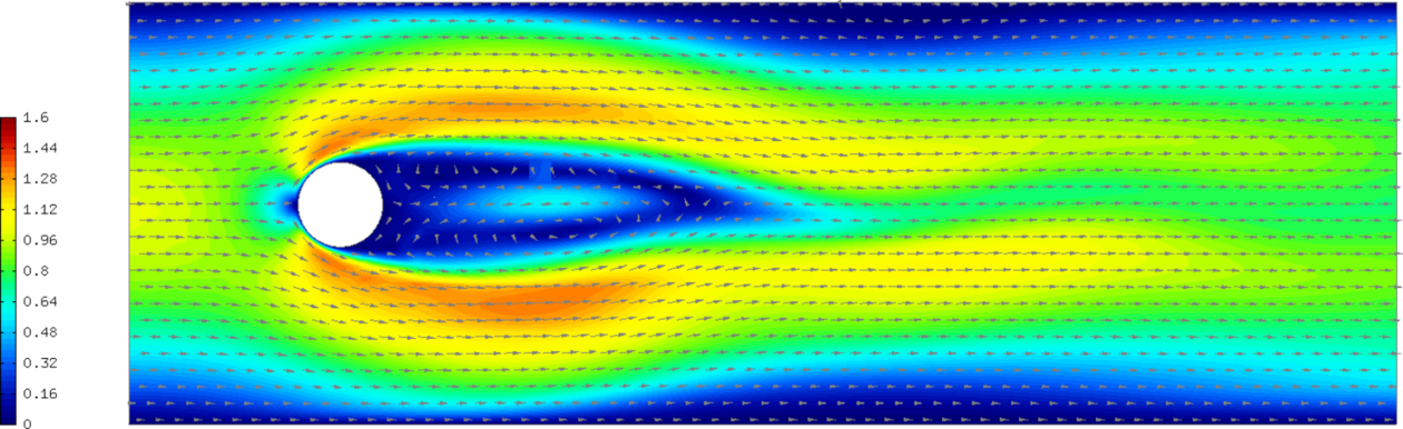
Sample results
The following comparisons demonstrate the effect of using the Newton’s method, and of using continuous vs. discontinuous elements for the pressure. There are three triplets of velocity snapshots. In each one, the images were obtained with (1) NEWTON == false && PRESSURE_IN_L2 undefined, (2) NEWTON == true && PRESSURE_IN_L2 undefined, and (3) NEWTON == true && PRESSURE_IN_L2 defined. It follows from these comparisons that one should definitely use the option (3).
Time t = 10 s:
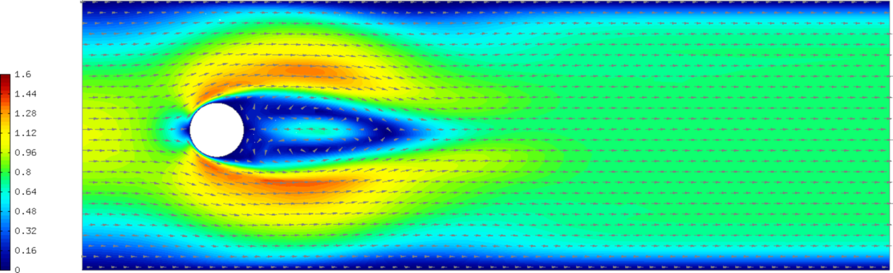
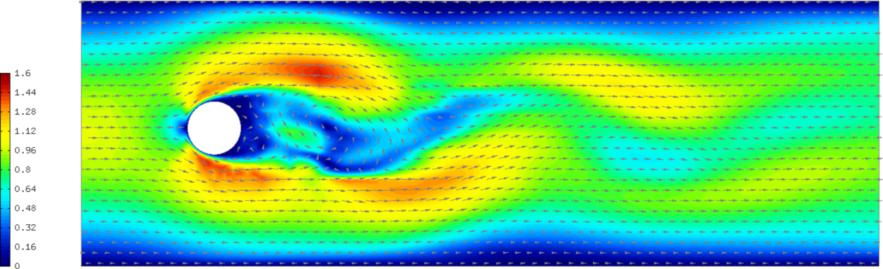
Time t = 15 s:
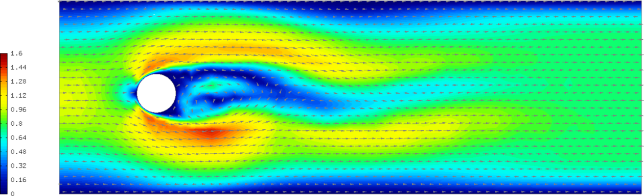
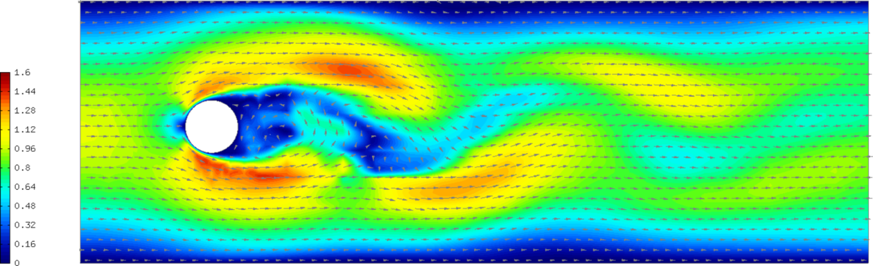
Time t = 21 s:
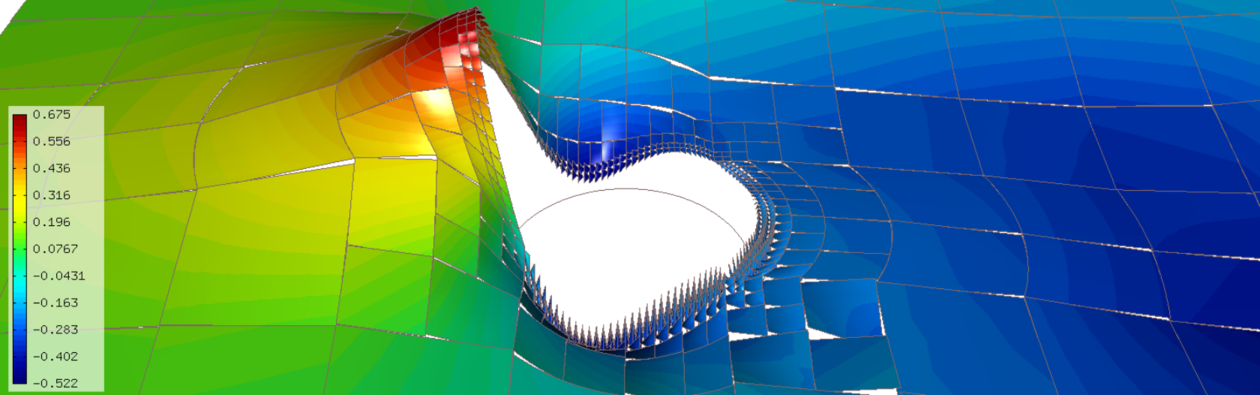
Snapshot of a continuous pressure approximation (t = 20 s):
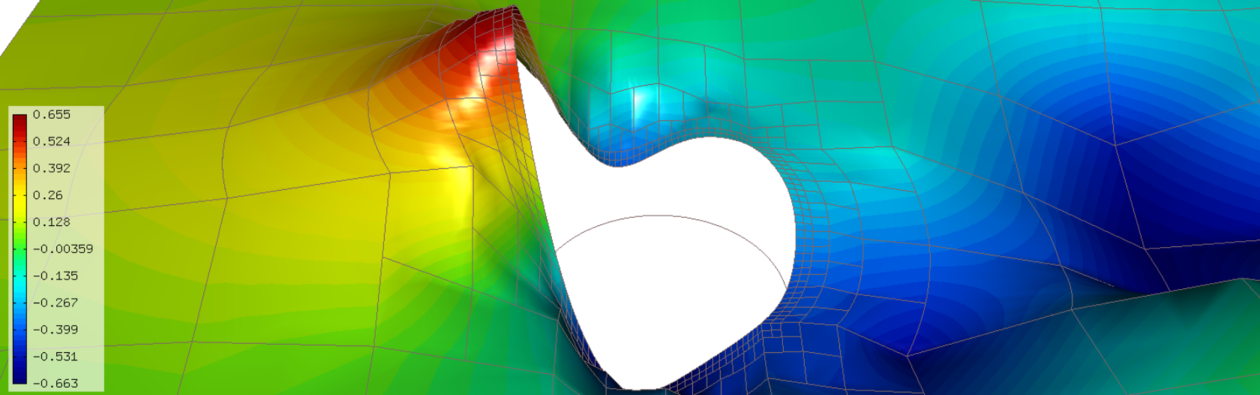
Snapshot of a discontinuous pressure approximation (t = 20 s):