Waveguide
By David Panek, University of West Bohemia, Czech Republic.
Mathematical description of waveguides
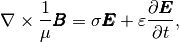
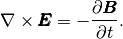
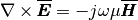
Mathematical description of waveguides is given by the Maxwell’s equations
(1)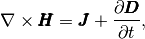
(2)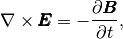
(3)
(4)
where
(5)
Here  means permittivity,
  permeability and
  stands for electric conductivity. For waveguides analysis, material properties are often considered constant and isotropic. After substituting material properties (5) into equations (1) and (2), we get
(6)
(7)
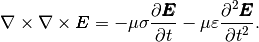
If the vector operator  is applied on the equation (7), it is possible to substitute
  from the equation (6) and get the wave equation for the electric field in the form
(8)
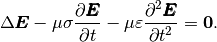
In a medium with zero charge density  it is useful to apply the vector identity
(9)
Since  ), the wave equation (8) can be
simplified to
), the wave equation (8) can be
simplified to
(10)
For many technical problems it is sufficient to know the solution in the frequency domain. After applying the Fourier transform, equation (10) becomes
(11)
which is the Helmholtz equation.
Decomposition into two real equations
The electric field  can be written as
(12)
Substituting into the original equation, we obtain
(13)
Last, comparing the real and imaginary numbers in the equation, we have
(14)
and
(15)
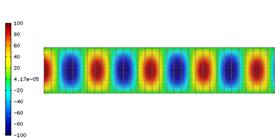
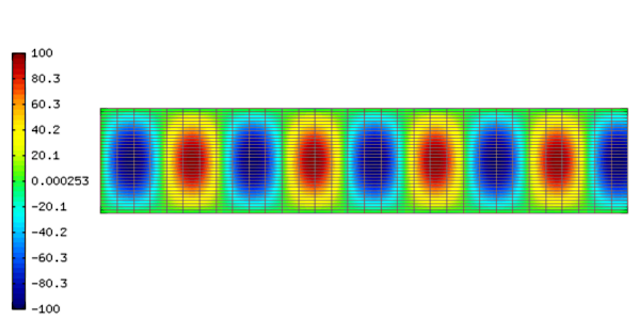
Parallel plate waveguide
Parallel plate waveguide is the simplest type of guide that supports TM (transversal magnetic) and TE (transversal electric) modes. This kind of guide allows also TEM (transversal electric and magnetic) mode.
Mathematical model - TE modes
Suppose that the electromagnetic wave is propagating in the direction  , then the component of the vector
  in the direction of the propagation is equal to zero
(16)
thus it is possible to solve the electric field in the parallel plate waveguide as a two-dimensional Helmholtz problem
(17)
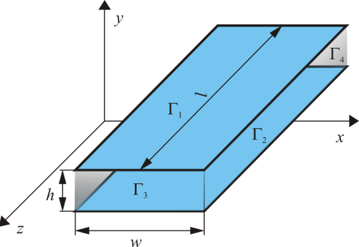
The conducting plates (boundary  ) are usually supposed to be perfectly conductive,
which can be modeled using the perfect conductor boundary condition
) are usually supposed to be perfectly conductive,
which can be modeled using the perfect conductor boundary condition
(18)
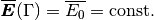
For the geometry in the above figure the expression (18) is reduced to a zero Dirichlet boundary condition
(19)
For the boundaries  , the following types of boundary conditions
can be used:
, the following types of boundary conditions
can be used:
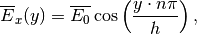
Electric field (Dirichlet boundary condition)
(20)
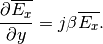
Note that for TE modes (and for the geometry shown above), a natural boundary condition is described by the expression
(21)
where  stands for a mode.
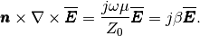
Impedance matching (Newton boundary condition)
For harmonic TE mode waves the following relation holds:
(22)

where  is the wave impedance. At the same time the second Maxwell equation
(23)
must be satisfied. From quations (22) and (23) it is possible to derive impedance matching boundary condition in the form
(24)
For a given geometry the equation (24) can be reduced to the Newton boundary condition in the form
(25)
Material parameters
const double epsr = 1.0;                    // Relative permittivity
const double eps0 = 8.85418782e-12;         // Permittivity of vacuum F/m
const double mur = 1.0;                     // Relative permeablity
const double mu0 = 4*M_PI*1e-7;             // Permeability of vacuum H/m
const double frequency = 3e9;               // Frequency MHz
const double omega = 2*M_PI * frequency;    // Angular velocity
const double sigma = 0;                     // Conductivity Ohm/m
Boundary conditions
There are three possible types of boundary conditions:
- Zero Dirichlet boundary conditions.
- Nonzero Dirichlet boundary conditions.
- Newton boundary conditions.