Boundary Layer (Elliptic)

This example is a singularly perturbed problem with known exact solution that exhibits a thin boundary layer The reader can use it to perform various experiments with adaptivity. The sample numerical results presented below imply that:

• One should always use anisotropically refined meshes for problems with boundary layers.
• hp-FEM is vastly superior to h-FEM with linear and quadratic elements.
• One should use not only spatially anisotropic elements, but also polynomial anisotropy (different polynomial orders in each direction) for problems in boundary layers.

Model problem

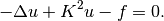
Equation solved: Poisson equation

(1)

Domain of interest: Square .

Boundary conditions: zero Dirichlet.

Exact solution

where is the exact solution of the 1D singularly-perturbed problem

in with zero Dirichlet boundary conditions. This solution has the form

Right-hand side

Calculated by inserting the exact solution into the equation.

Sample solution

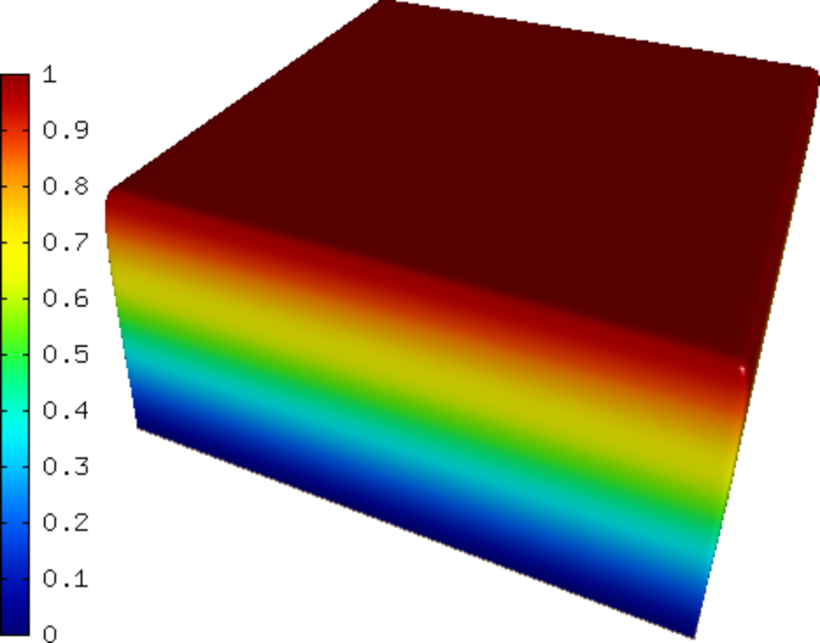
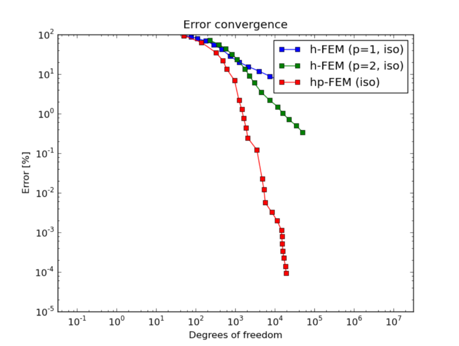
Below we present a series of convergence comparisons. Note that the error plotted is the true approximate error calculated wrt. the exact solution given above.

Convergence comparison for isotropic refinements

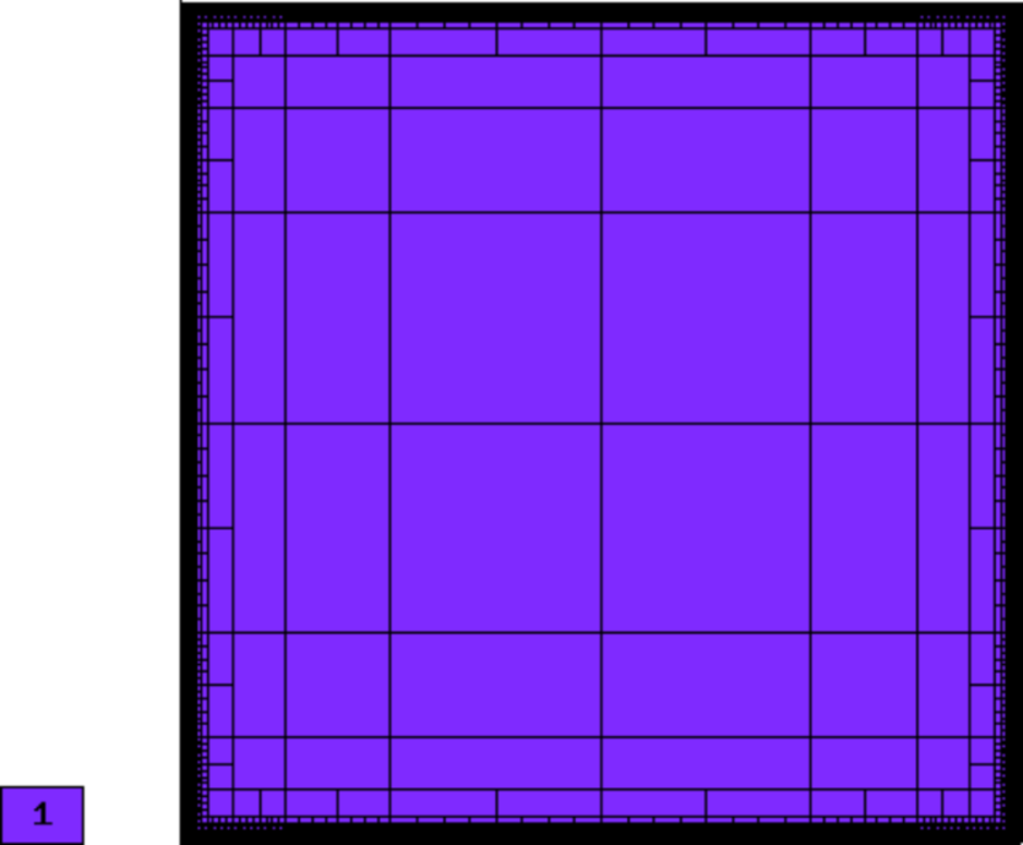
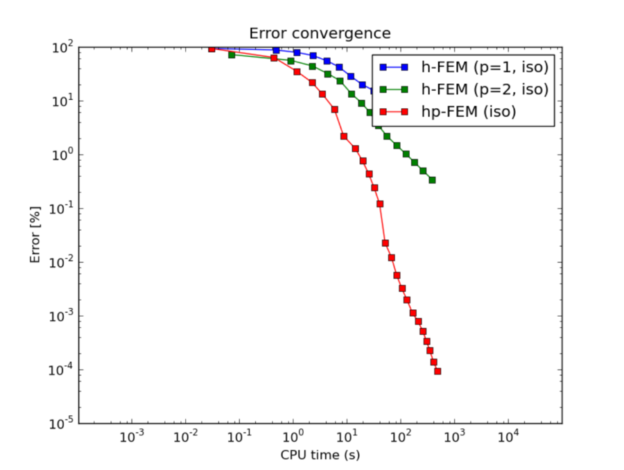
Let us first compare the performance of h-FEM (p=1), h-FEM (p=2) and hp-FEM with isotropic refinements:

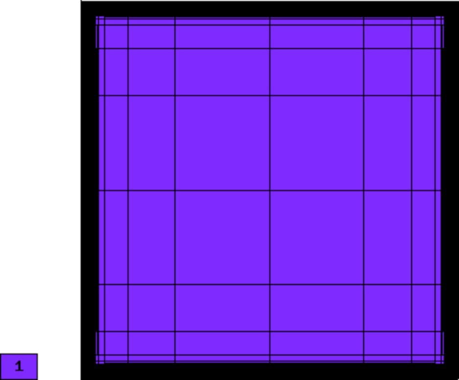
Final mesh (h-FEM, p=1, isotropic refinements):

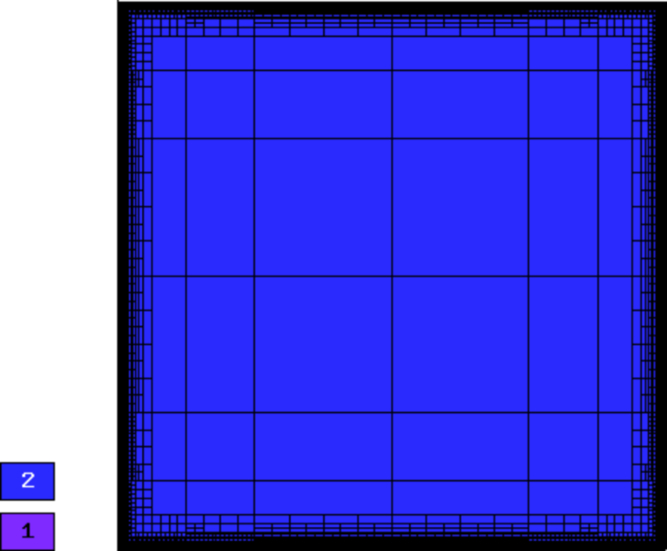
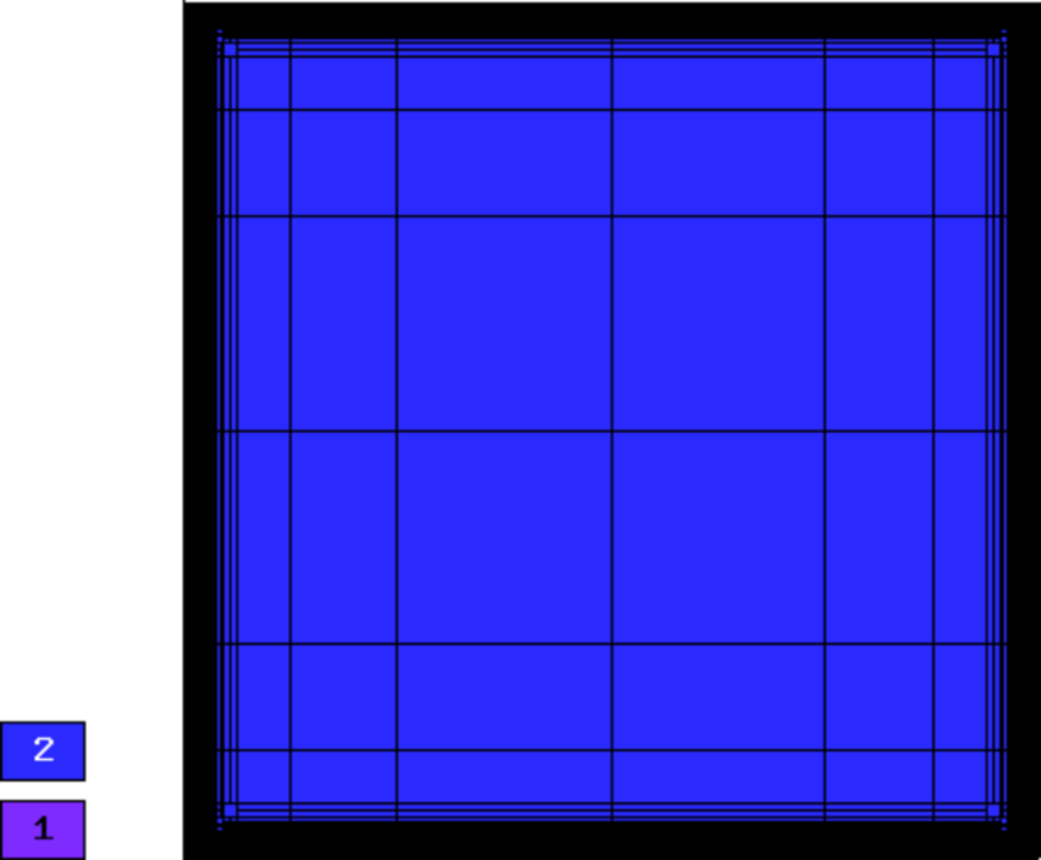
Final mesh (h-FEM, p=2, isotropic refinements):

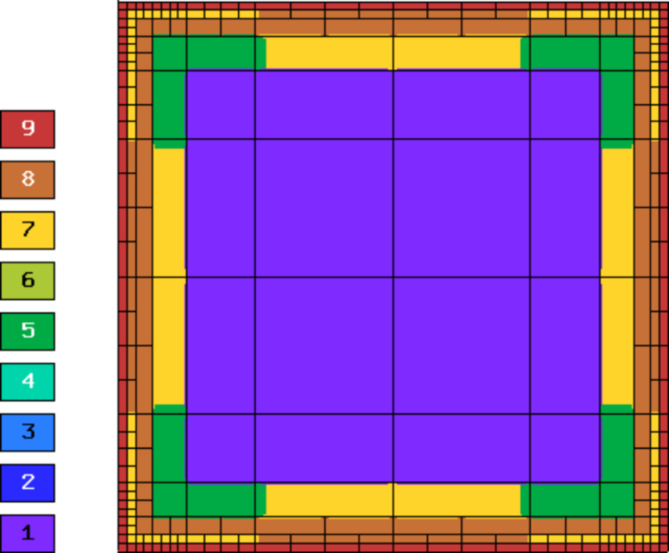
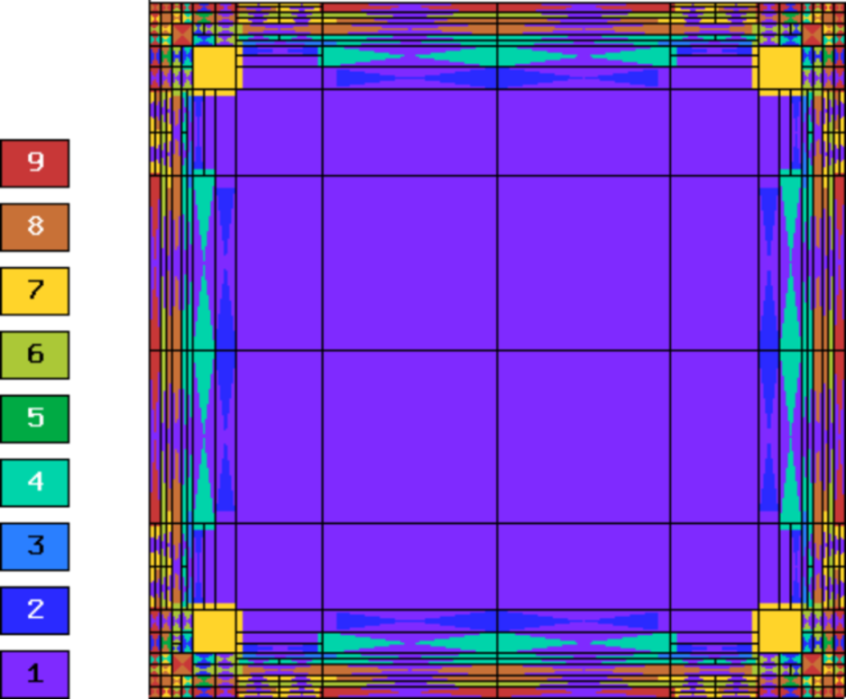
Final mesh (hp-FEM, isotropic refinements):

DOF convergence graphs:

CPU convergence graphs:

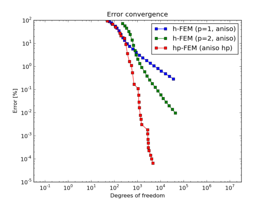
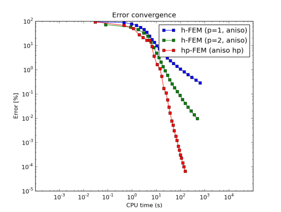
Convergence comparison for anisotropic refinements

Next we compare the performance of h-FEM (p=1), h-FEM (p=2) and hp-FEM with anisotropic refinements:

Final mesh (h-FEM, p=1, anisotropic refinements):

Final mesh (h-FEM, p=2, anisotropic refinements):

Final mesh (hp-FEM, anisotropic refinements):

DOF convergence graphs:

CPU convergence graphs:

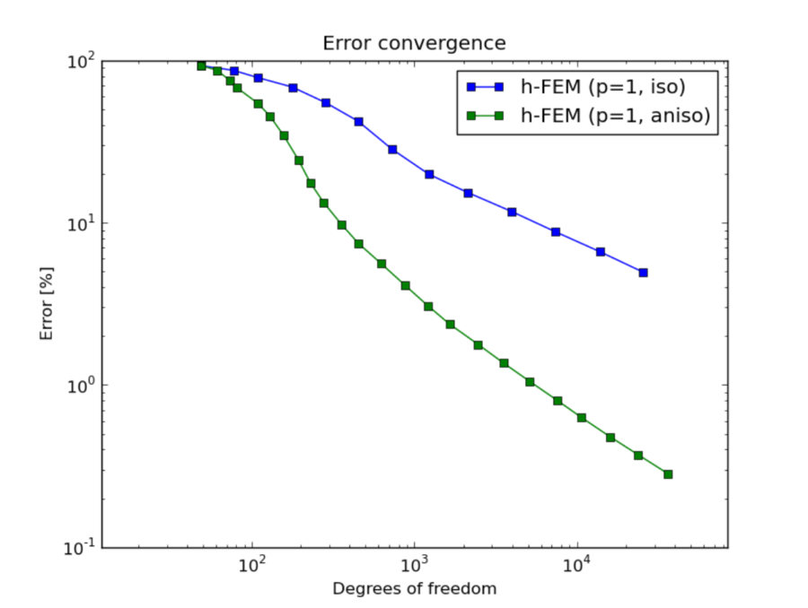
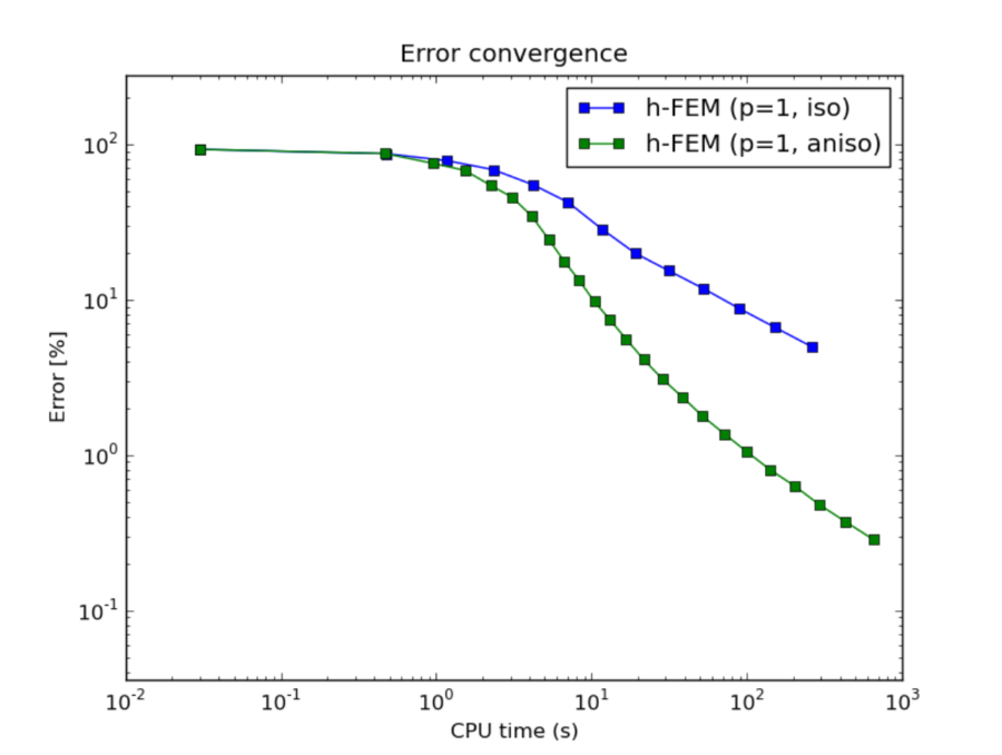
h-FEM (p=1): comparison of isotropic and anisotropic refinements

DOF convergence graphs:

CPU convergence graphs:

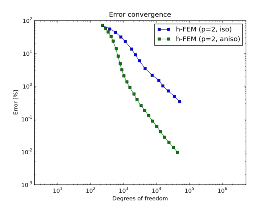
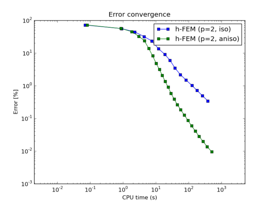
h-FEM (p=2): comparison of isotropic and anisotropic refinements

DOF convergence graphs:

CPU convergence graphs:

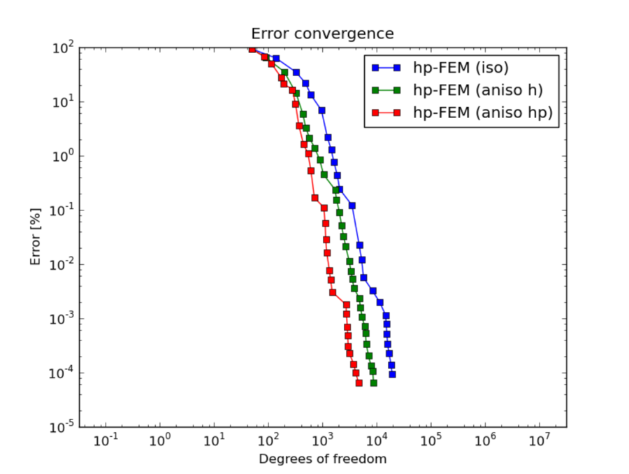
hp-FEM: comparison of isotropic and anisotropic refinements

In the hp-FEM one has two kinds of anisotropy – spatial and polynomial. In the following, “iso” means isotropy both in h and p, “aniso h” means anisotropy in h only, and “aniso hp” means anisotropy in both h and p.

DOF convergence graphs (hp-FEM):

CPU convergence graphs (hp-FEM):

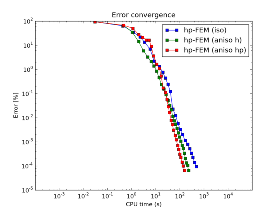
The reader can see that enabling polynomially anisotropic refinements in the hp-FEM is equally important as allowing spatially anisotropic ones.