Space H(curl) (03-space-hcurl)

In the tutorial example “P01-linear/02-space” we first saw how a finite element space over a mesh is created. That was an H1 space suitable for continuous approximations. Another widely used Sobolev space, H(curl), is typically present in Maxwell’s problems of electromagnetics. H(curl) approximations are discontinuous, elementwise polynomial vector fields that behave like gradients of H1 functions. Recall that in electrostatics In particular, H(curl) functions have continuous tangential components along all mesh edges. For the application of the H(curl) space check examples related to Maxwell’s equations in the previous sections. Below is a simple code that shows how to set up an H(curl) space and visualize its finite element basis functions:

int INIT_REF_NUM = 2;      // Initial uniform mesh refinement.
int P_INIT = 3;            // Polynomial degree of mesh elements.

int main(int argc, char* argv[])
{
  // Load the mesh.
  Mesh mesh;
  MeshReaderH2D mloader;
  mloader.load("square.mesh", &mesh);

  // Initial mesh refinement.
  for (int i = 0; i < INIT_REF_NUM; i++) mesh.refine_all_elements();

  HcurlSpace<double> space(&mesh, P_INIT);

  // Visualize FE basis.
  VectorBaseView<double> bview("VectorBaseView", new WinGeom(0, 0, 700, 600));
  bview.show(&space);

  // Wait for all views to be closed.
  View::wait();
  return 0;
}

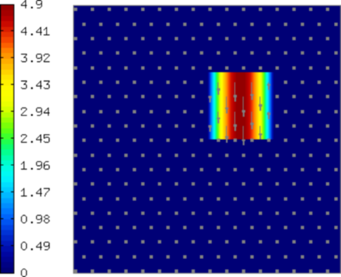
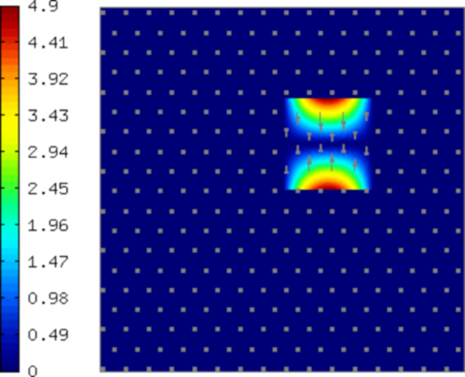
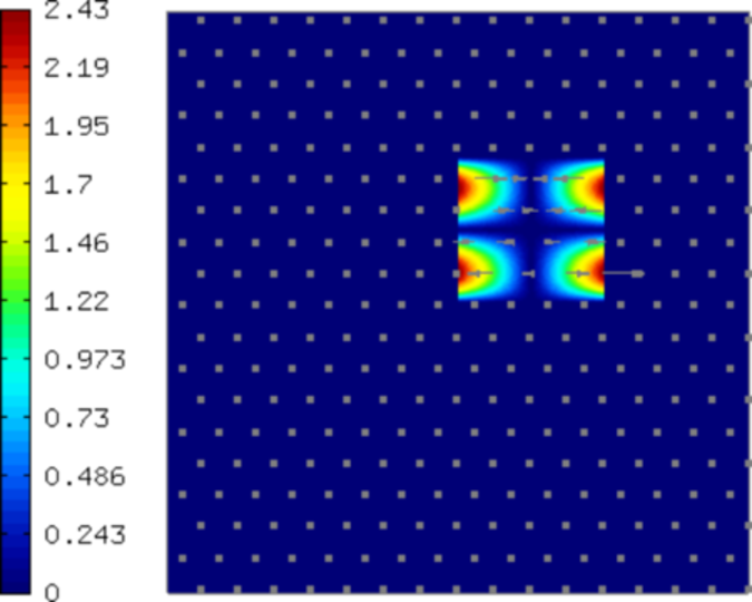
The class VectorBaseView allows the user to browse through the finite element basis functions using the left and right arrows. A few sample basis functions (higher-order bubble functions) are shown below. The color shows magnitude of the vector field, arrows show its direction.

The space H(curl) is implemented for both quadrilateral and triangular elements, and both element types can be combined.