Newton’s Method and Adaptivity (07-nonlinear)

In this example we use the nonlinear model problem from example “P02-nonlinear/02-newton-spline”,

equipped with nonhomogeneous Dirichlet boundary conditions

This time it will be solved using automatic adaptivity.

Initial solve on coarse mesh

First we calculate an initial coefficient vector by projecting the initial condition on the coarse mesh:

InitialSolutionHeatTransfer init_sln(&mesh);
OGProjection<double> ogProjection; ogProjection.project_global(&space, &init_sln, coeff_vec_coarse);

Then we solve the problem on the coarse mesh:

// Perform initial Newton's iteration on coarse mesh, to obtain
// good initial guess for the Newton's method on the fine mesh.
try
{
  newton_coarse.solve(coeff_vec_coarse);
}
catch(Hermes::Exceptions::Exception e)
{
  e.printMsg();

}

The resulting coefficient vector is translated into a coarse mesh solution:

// Translate the resulting coefficient vector into the Solution<double> sln.
Solution<double>::vector_to_solution(newton_coarse.get_sln_vector(), &space, &sln);

Calculating initial coefficient vector on the reference mesh

In the adaptivity loop, we project the best approximation we have to obtain an initial coefficient vector on the new fine mesh. This step is quite important since the reference space is large, and the quality of the initial coefficient vector matters a lot. In the first adaptivity step, we use the coarse mesh solution (that’s why we have computed it), and in all other steps we use the previous fine mesh solution:

// Calculate initial coefficient vector on the reference mesh.
double* coeff_vec = new double[Space<double>::get_num_dofs(ref_space)];
if (as == 1)
{
  // In the first step, project the coarse mesh solution.
  info("Projecting coarse mesh solution to obtain initial vector on new fine mesh.");
  OGProjection<double> ogProjection; ogProjection.project_global(ref_space, &sln, coeff_vec);
}
else
{
  // In all other steps, project the previous fine mesh solution.
  info("Projecting previous fine mesh solution to obtain initial vector on new fine mesh.");
  OGProjection<double> ogProjection; ogProjection.project_global(ref_space, &ref_sln, coeff_vec);
}

Sample results

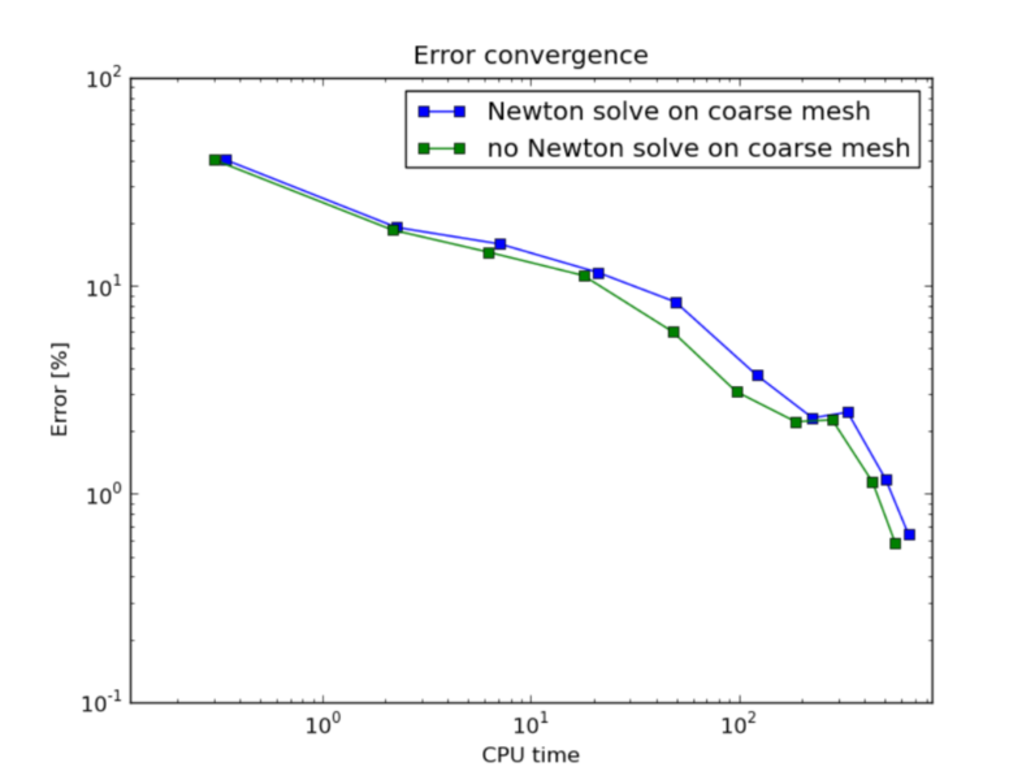
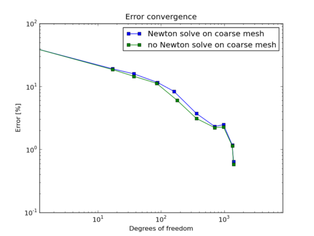
We performed an experiment where we used on the coarse mesh (a) orthogonal projection of the fine mesh solution and (b) we solved the nonlinear problem on the coarse mesh. We found that this difference does not affect convergence significantly, as illustrated in the following convergence comparisons.

1. Convergence in the number of DOF (with and without Newton solve on the new coarse mesh):

2. Convergence in CPU time (with and without Newton solve on coarse mesh):