Complex-Valued Problem (04-complex)

This example shows how to define complex-valued weak forms, essential boundary conditions, spaces, solutions, discrete problem, and how to perform orthogonal projection and adaptivity in complex mode. In addition, it shows how to use the AZTECOO matrix solver (other solvers including UMFPACK can be used as well - use them if you do not have Trilinos installed). Installation of matrix solvers including Trilinos is described in detail in the library documentation.

Model problem

We solve a complex-valued vector potential problem

in a two-dimensional cross-section containing a conductor and an iron object. Note: in 2D this is a double problem. A sketch of the computational domain is shown in the following picture:

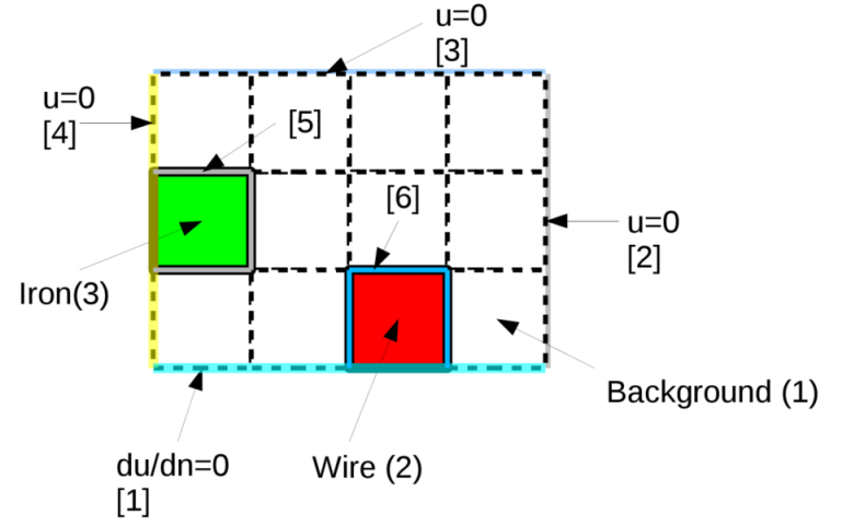
The computational domain is a rectangle of height 0.003 and width 0.004. Different material markers are used for the wire, air, and iron (see mesh file “domain.mesh”).

Boundary conditions are zero Dirichlet on the top and right edges, and zero Neumann elsewhere.

Complex-valued weak forms

The weak formulation consists entirely of default forms, its header looks as follows:

class CustomWeakForm<double> : public WeakForm<std::complex<double> >
{
public:
  CustomWeakForm(std::string mat_air,  double mu_air,
                 std::string mat_iron, double mu_iron, double gamma_iron,
                 std::string mat_wire, double mu_wire, std::complex<double> j_ext, double omega);
};

For details see the files definitions.h and definitions.cpp.

Defining complex essential BCs

This is analogous to defining real-valued BCs, except that the type “std::complex<double>” is used in the template instead of “double”:

// Initialize boundary conditions.
Hermes::Hermes2D::DefaultEssentialBCConst<std::complex<double> >
  bc_essential("Dirichlet", std::complex<double>(0.0, 0.0));
EssentialBCs<std::complex<double> > bcs(&bc_essential);

Defining a complex H1 space

This is analogous to defining a real-valued H1 space:

H1Space<std::complex<double> > space(&mesh, &bcs, P_INIT);

All other templated objects are treated analogously, see the file main.cpp for more details.

Initializing the AztecOO matrix solver

Inside the adaptivity loop, the matrix solver is initialized as follows:

// For iterative solver.
if (matrix_solver == SOLVER_AZTECOO)
{
  newton.set_iterative_method(iterative_method);
  newton.set_preconditioner(preconditioner);
}

Here, “iterative_method” and “preconditioner” have been defined at the beginning of the file main.cpp.

Otherwise everything works as usual.

Sample results

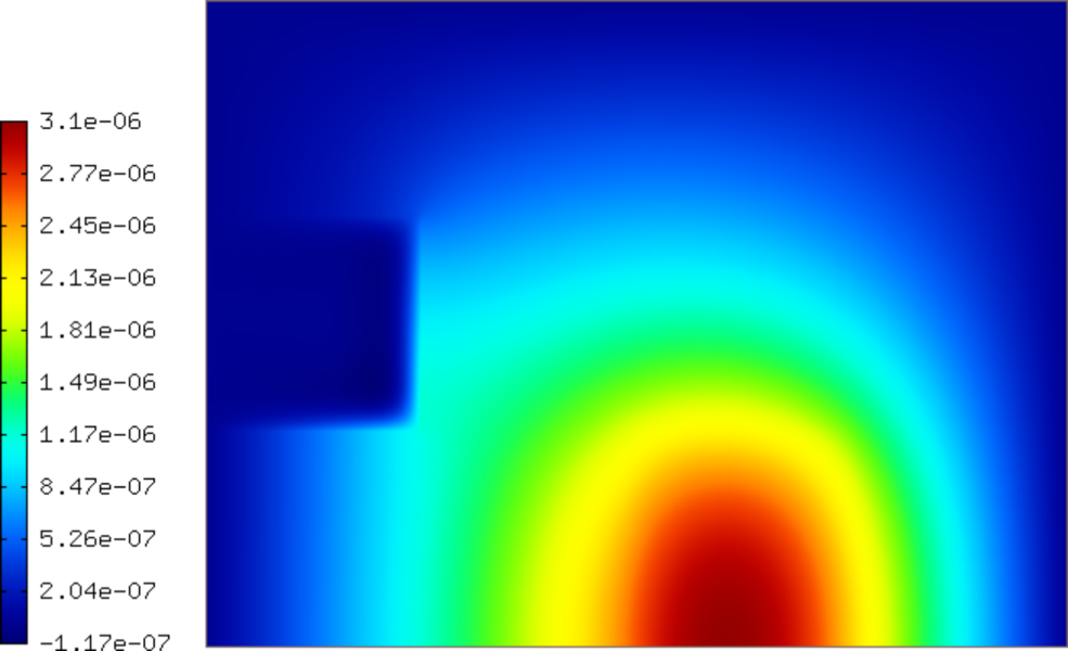
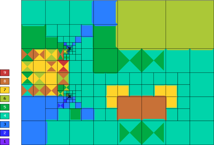
Solution:

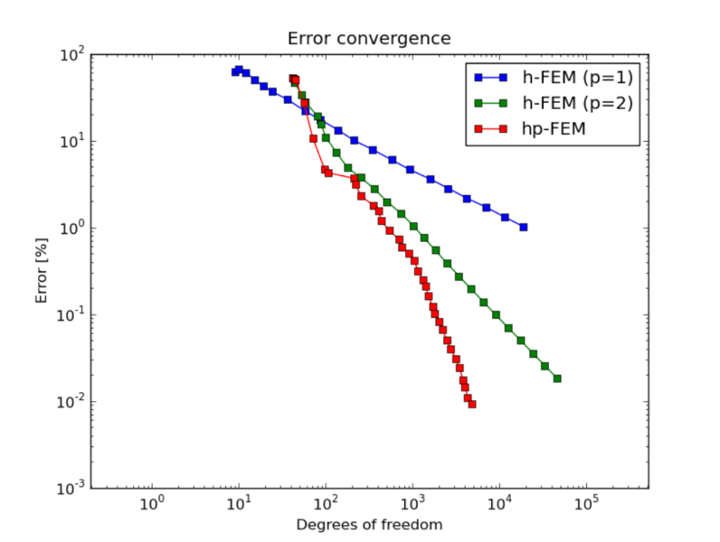
Let us compare adaptive h-FEM with linear and quadratic elements and the hp-FEM.

Final mesh for h-FEM with linear elements: 18694 DOF, error = 1.02 %

Final mesh for h-FEM with quadratic elements: 46038 DOF, error = 0.018 %

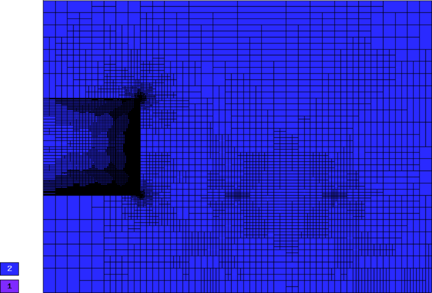
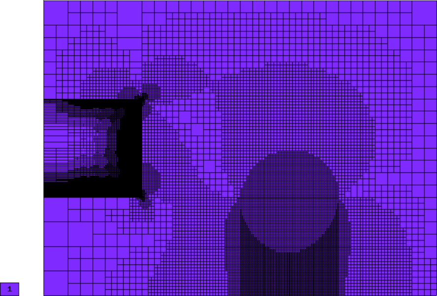
Final mesh for hp-FEM: 4787 DOF, error = 0.00918 %

Convergence graphs of adaptive h-FEM with linear elements, h-FEM with quadratic elements and hp-FEM are shown below.