Basic-rk-newton-adapt
Model problem
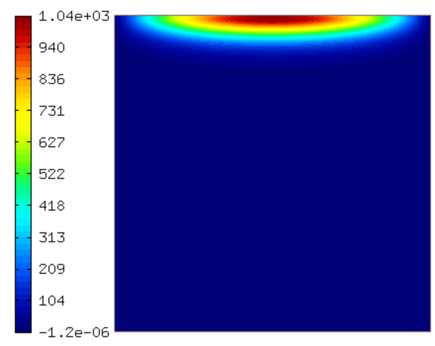
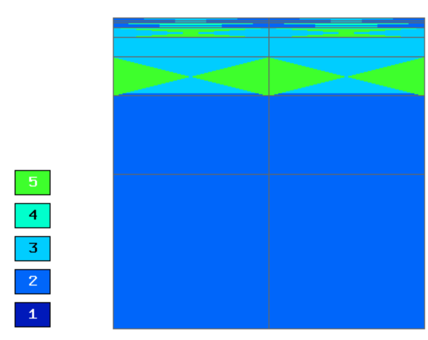
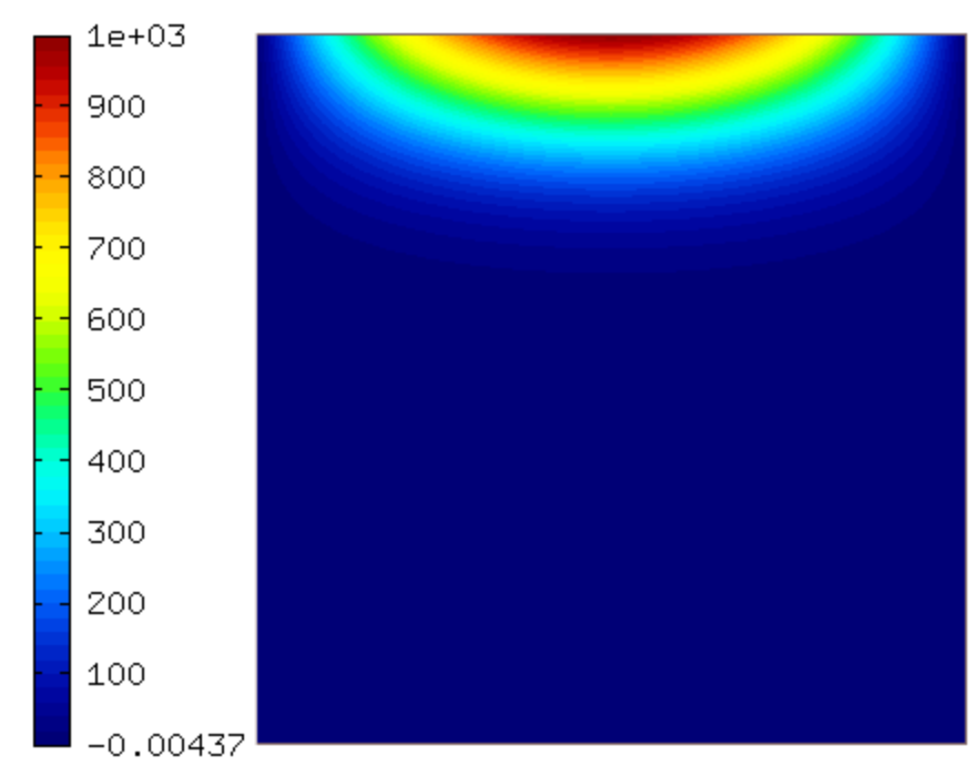
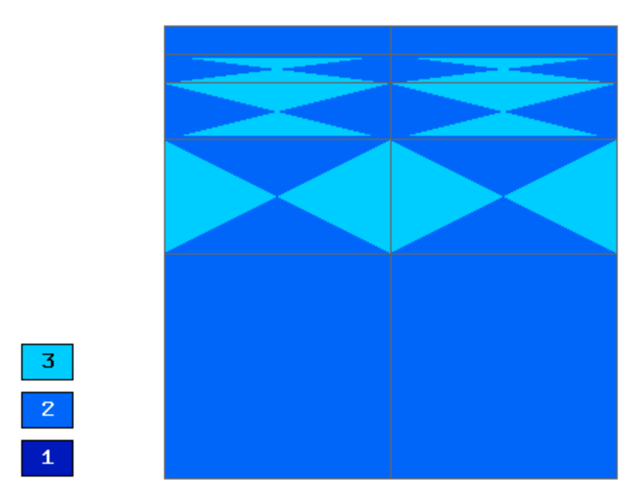
This example uses adaptivity with dynamical meshes to solve the Tracy problem with arbitrary Runge-Kutta methods in time.
We assume the time-dependent Richard’s equation
(1)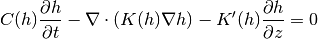
where  and
and  are given functions of the unknown pressure head
  ,
,  are spatial coordinates, and
  is time.
equipped with a Dirichlet, given by the initial condition.

The pressure head ‘h’ is between -1000 and 0. For convenience, we increase it by an offset H_OFFSET = 1000. In this way we can start from a zero coefficient vector.

Defining weak forms
The weak formulation is a combination of custom Jacobian and Residual weak forms:
CustomWeakFormRichardsRK::CustomWeakFormRichardsRK() : WeakForm<double>(1)
{
  // Jacobian volumetric part.
  CustomJacobianFormVol* jac_form_vol = new CustomJacobianFormVol(0, 0);
  add_matrix_form(jac_form_vol);

  // Residual - volumetric.
  CustomResidualFormVol* res_form_vol = new CustomResidualFormVol(0);
  add_vector_form(res_form_vol);
}