Laminar Flame
Problem description
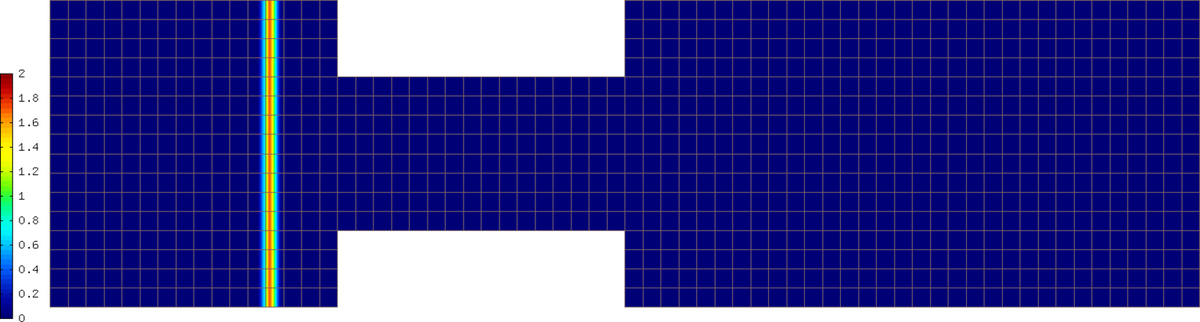
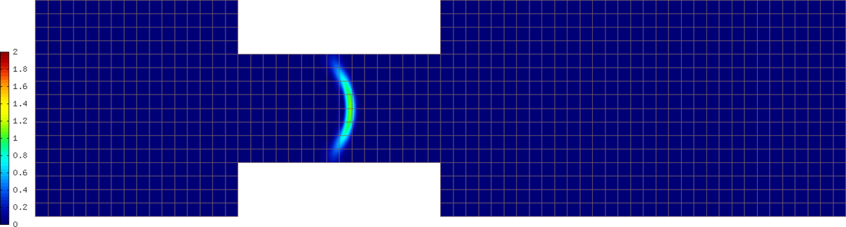
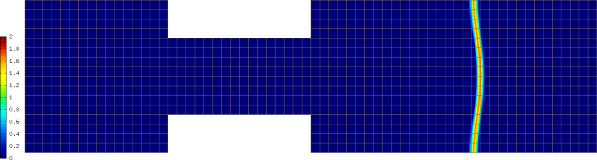
We will employ the Newton’s method to solve a nonlinear system of two parabolic equations describing a very simple flame propagation model (laminar flame, no fluid mechanics involved). The computational domain shown below contains in the middle a narrow portion (cooling rods) whose purpose is to slow down the chemical reaction:

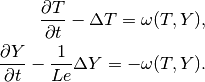
The equations for the temperature  and species concentration
  have the form
Boundary conditions are Dirichlet  and
and  on the inlet,
Newton
on the inlet,
Newton 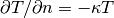 on the cooling rods,
and Neumann
on the cooling rods,
and Neumann  ,
,  elsewhere.
The objective of the computation is to obtain the reaction rate defined
by the Arrhenius law,
elsewhere.
The objective of the computation is to obtain the reaction rate defined
by the Arrhenius law,
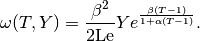
Here  is the gas expansion coefficient in a flow with nonconstant density,
 the non-dimensional activation energy, and
 the Lewis number (ratio of diffusivity of heat and diffusivity
of mass). Both
the Lewis number (ratio of diffusivity of heat and diffusivity
of mass). Both  ,
,  and
,
and
,  are dimensionless and so is the time
  .
.
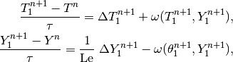
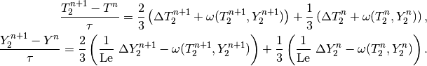
Second-order BDF formula for time integration
Time integration is performed using a second-order implicit BDF formula
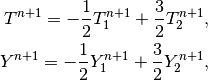
that is obtained using a combination of the following two first-order methods:
and
Problem parameters are chosen as
// Problem constants
const double Le    = 1.0;
const double alpha = 0.8;
const double beta  = 10.0;
const double kappa = 0.1;
const double x1 = 9.0;
Initial conditions
It is worth mentioning that the initial conditions for and ,
// Initial conditions.
scalar temp_ic(double x, double y, scalar& dx, scalar& dy)
  { return (x <= x1) ? 1.0 : exp(x1 - x); }

scalar conc_ic(double x, double y, scalar& dx, scalar& dy)
  { return (x <= x1) ? 0.0 : 1.0 - exp(Le*(x1 - x)); }
are defined as exact functions:
// Set initial conditions.
t_prev_time_1.set_exact(&mesh, temp_ic); c_prev_time_1.set_exact(&mesh, conc_ic);
t_prev_time_2.set_exact(&mesh, temp_ic); c_prev_time_2.set_exact(&mesh, conc_ic);
t_prev_newton.set_exact(&mesh, temp_ic);  c_prev_newton.set_exact(&mesh, conc_ic);
Here the pairs of solutions (t_prev_time_1, y_prev_time_1) and (t_prev_time_2, y_prev_time_2) correspond to the two first-order time-stepping methods described above. and (t_prev_newton, y_prev_newton) are used to store the previous step approximation in the Newton’s method.
Using Filters
The reaction rate  and its derivatives are handled
via Filters:
and its derivatives are handled
via Filters:
// Filters for the reaction rate omega and its derivatives.
DXDYFilter omega(omega_fn, Tuple<MeshFunction*>(&t_prev_newton, &c_prev_newton));
DXDYFilter omega_dt(omega_dt_fn, Tuple<MeshFunction*>(&t_prev_newton, &c_prev_newton));
DXDYFilter omega_dc(omega_dc_fn, Tuple<MeshFunction*>(&t_prev_newton, &c_prev_newton));
Details on the functions omega_fn, omega_dt_fn, omega_dy_fn and the weak forms can be found in the file forms.cpp
Reinitialization of Filters
Notice the reinitialization of the Filters at the end of the Newton’s loop. This is necessary as the functions defining the Filter have changed:
// Set current solutions to the latest Newton iterate
// and reinitialize filters of these solutions.
Solution::vector_to_solutions(newton.get_sln_vector(), Tuple<Space *>(&tspace, &cspace),
                              Tuple<Solution *>(&t_prev_newton, &c_prev_newton));
omega.reinit();
omega_dt.reinit();
omega_dc.reinit();
Visualization of a Filter
Also notice the visualization of a Filter:
// Visualization.
DXDYFilter omega_view(omega_fn, Tuple<MeshFunction*>(&t_prev_newton, &c_prev_newton));
rview.set_min_max_range(0.0,2.0);
char title[100];
sprintf(title, "Reaction rate, t = %g", current_time);
rview.set_title(title);
rview.show(&omega_view);