Linear Advection-Diffusion
Problem description
This example solves the equation
in the domain  where
where  is the diffusivity and
  a constant advection velocity. We assume that
  and
and  . The boundary
conditions are Dirichlet.
. The boundary
conditions are Dirichlet.
With a small  , this is a singularly
perturbed problem whose solution is close to 1 in most of the domain and forms
a thin boundary layer along the top
and right edges of
, this is a singularly
perturbed problem whose solution is close to 1 in most of the domain and forms
a thin boundary layer along the top
and right edges of  .
.
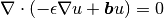
Solution for  . Note - view selected to show the boundary layer:
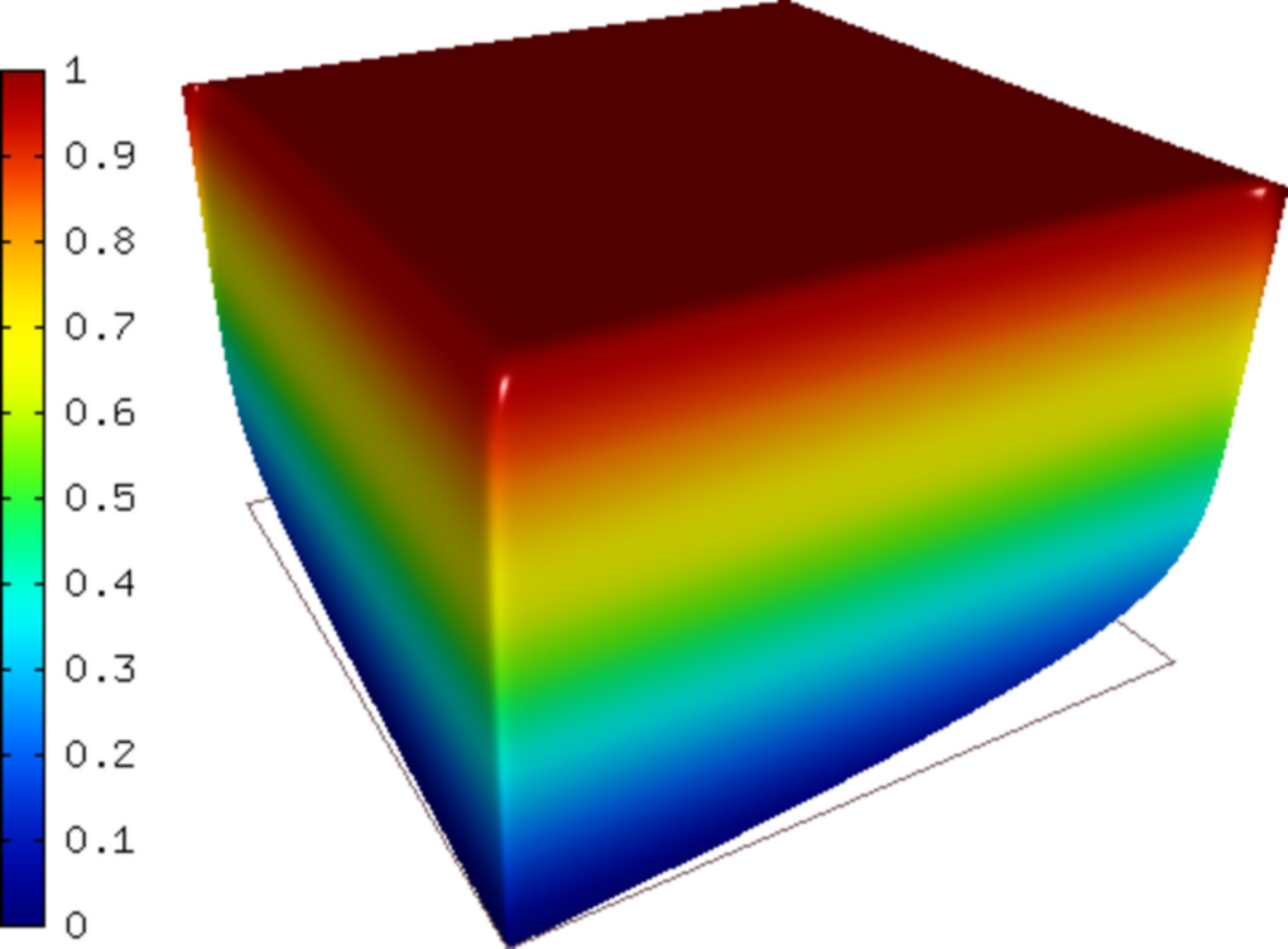
Initial mesh for automatic adaptivity:
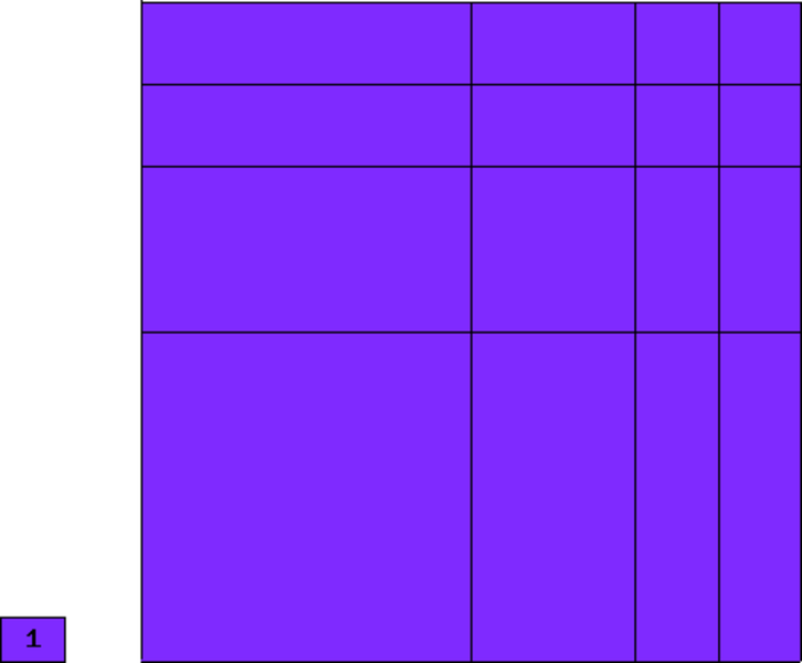
This mesh is not fine enough in the boundary layer region to prevent the solution from oscillating:
Here we use the same view as for the solution above. As you can see, this approximation is not very close to the final solution. The oscillations can be suppressed by applying the multiscale stabilization (STABILIZATION_ON = true):

Automatic adaptivity can sometimes take care of them as well, as we will see below. Standard stabilization techniques include SUPG, GLS and others. For this example, we implemented the so-called variational multiscale stabilization that can be used on an optional basis. We have also implemented a shock-capturing term for the reader to experiment with.
Sample results
The stabilization and shock capturing are turned off for this computation.
Let us compare adaptive  -FEM with linear and quadratic elements and the
  -FEM.
-FEM.
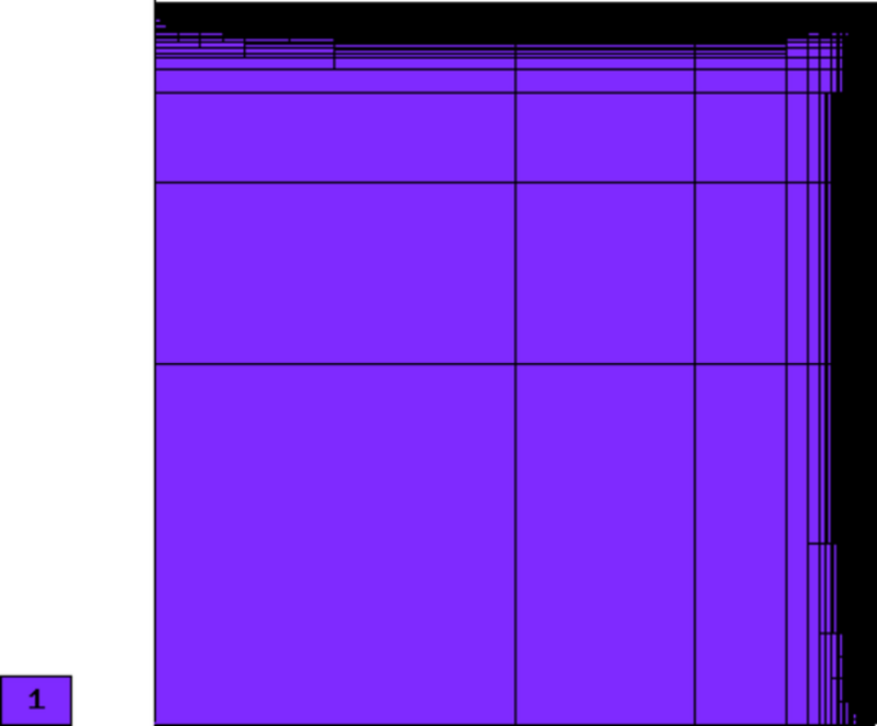
Final mesh for -FEM with linear elements: 57495 DOF, error = 0.66 %
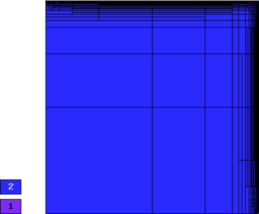
Final mesh for -FEM with quadratic elements: 4083 DOF, error = 0.37 %
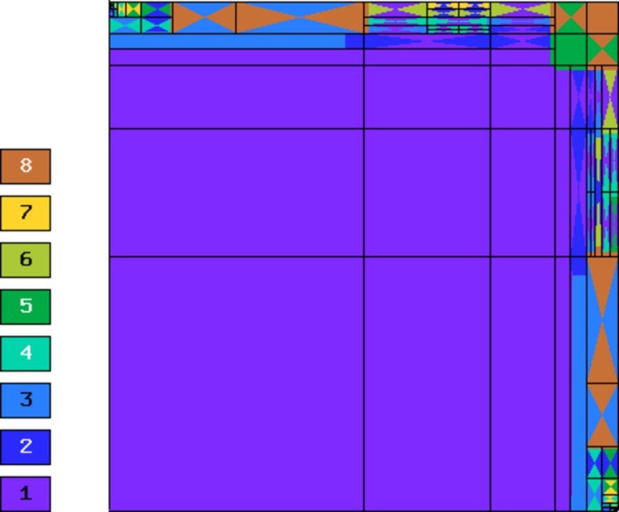
Final mesh for -FEM: 1854 DOF, error = 0.28 %
Convergence graphs of adaptive h-FEM with linear elements, h-FEM with quadratic elements and hp-FEM are shown below.
