NIST-07 (Boundary Line Singularity)
Many papers on testing adaptive algorithms use a 1D example with a singularity of the form  at the left endpoint of the domain. This can be extended to 2D by simply making the solution be
constant in
at the left endpoint of the domain. This can be extended to 2D by simply making the solution be
constant in  .
.
Model problem
Equation solved: Poisson equation
(1)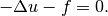
Domain of interest: Unit Square 
Boundary conditions: Dirichlet, given by exact solution.

 determines the strength of the singularity.
Right-hand side
Obtained by inserting the exact solution into the equation.
 :
:
Comparison of h-FEM (p=1), h-FEM (p=2) and hp-FEM with anisotropic refinements
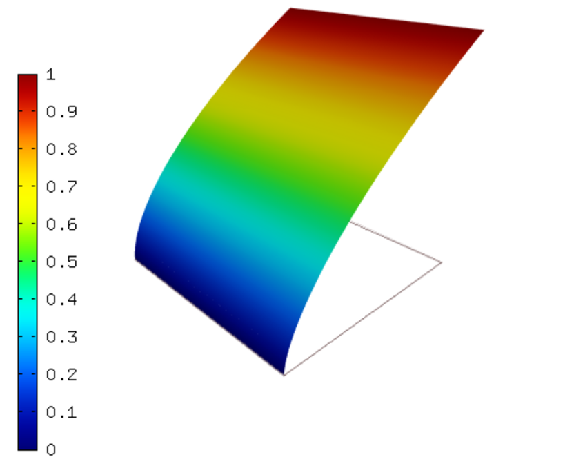
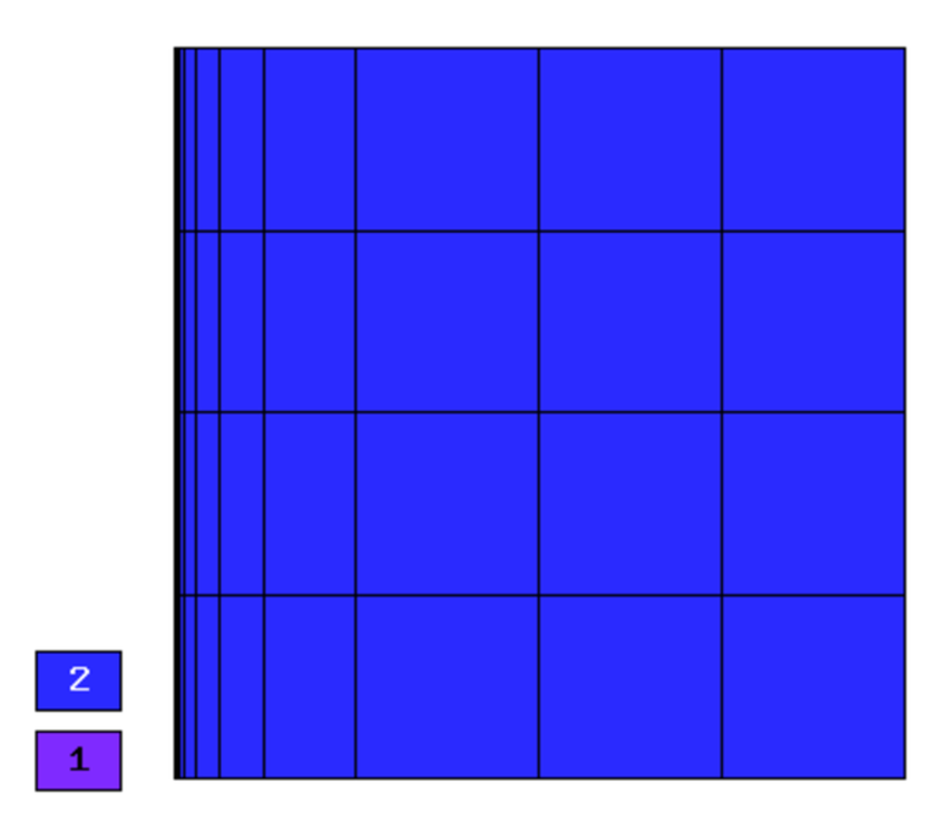
Final mesh (h-FEM, p=1, anisotropic refinements):
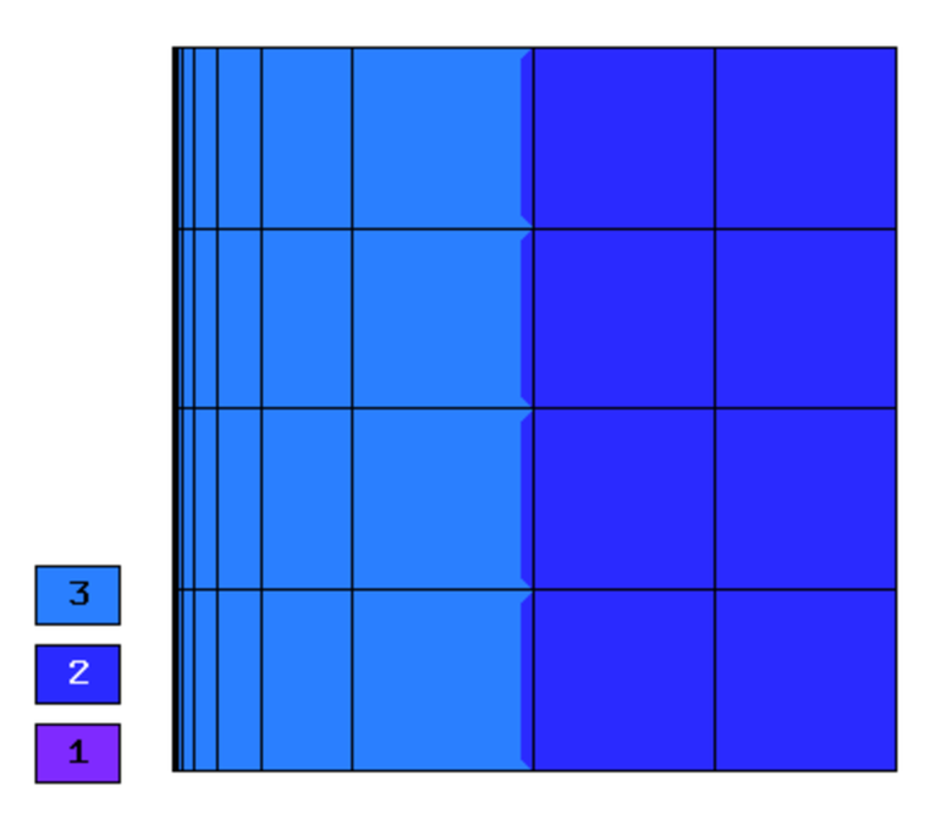
Final mesh (h-FEM, p=2, anisotropic refinements):
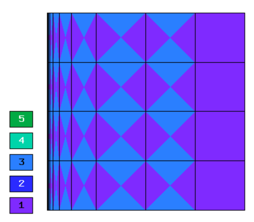
Final mesh (hp-FEM, h-anisotropic refinements):
DOF convergence graphs:

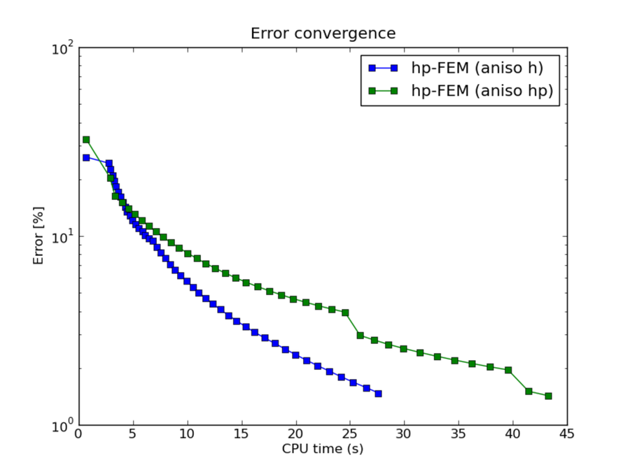
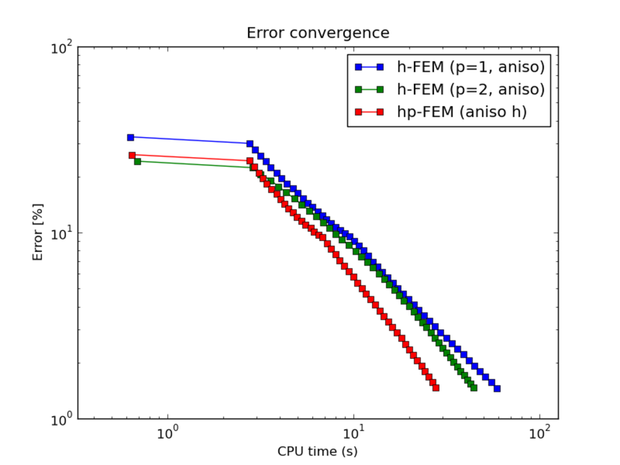
CPU convergence graphs:
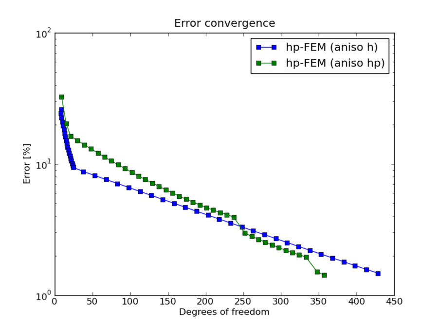
hp-FEM with h-aniso and hp-aniso refinements
Final mesh (hp-FEM, h-anisotropic refinements):
Final mesh (hp-FEM, hp-anisotropic refinements):
DOF convergence graphs:
CPU convergence graphs: